Example 8. Combined Sewer Systems in InfoSWMM and InfoSWMM SA

This example demonstrates how to model systems that convey both sanitary wastewater and stormwater through the same pipes. Systems like these are known as combined sewer systems and are still quite common in older communities and cities. During periods of moderate to heavy rainfall the capacity of these systems to convey and properly treat the combined flow can be exceeded, resulting in what are known as Combined Sewer Overflows (CSOs). CSO discharges can cause serious pollution problems in receiving waters. Contaminants from these discharges can include conventional pollutants, pathogens, toxic chemicals and debris.

This example will use H2OMAP SWMM to analyze the occurrence of overflows in a combined sewer system. Particular attention is paid to properly representing the flow regulators that divert flow between collection sewers, treatment plant interceptors and CSO outfalls. In addition, the example shows how to model a pump station that conveys the intercepted flow through a force main pipeline to the headworks of a treatment facility. Although the focus of this example is on combined systems, many of the same modeling elements it employs (wastewater inflows, pump stations, and force mains) can also be used to model separate sanitary sewer systems. See the accompanying ‘H2OMAP SWMM Applications.HSM’ model, scenario ‘EX8-COMBINED_SEWERS’ (with ‘child’ scenarios) for a complete worked out solution.

8.1 Problem Statement

Rather than being a new development, the 29 acre urban catchment studied in Example 2 (refer to ‘EX2-POST’ ‘parent’, ‘child’ and ‘grandchild’ scenarios in ‘H2OMAP SWMM Applications.HSM’) is now assumed to be an older area that is served by an existing combined sewer system. The hydraulic behavior of this combined system, including the magnitude of any overflows, will be analyzed for several different size storms. These include the 0.23 in. water quality storm defined in Example 3 as well as the 1.0 in., 2-yr and 1.7 in., 10-yr storms used throughout the previous examples.

Combined sewer pipes conveying both wastewater and stormwater flows generated within different sewersheds (i.e., areas that contribute wastewater flows to a single point) will be added to the model. Constant wastewater flows (also known as dry-weather flows) will be based on average generation rates per capita. An interceptor pipe will be sized to convey both the base dry weather flow and a portion of the combined stormwater flow to a pump station that pumps to the headworks of a wastewater treatment plant (WWTP) through a force main. Various combinations of orifices, weirs and pipes will be used to represent different types of flow diversion structures located within the interceptor. The CSOs that cannot be diverted by these devices will discharge directly into the stream running through the site’s park area.

The schematic representation of the combined sewer system modeled in this example is shown in Figure 8‑1. It includes the combined sewer pipes (in green) that drain the Subcatchments (or sewersheds) S1, S2, S3, S4 and S5, the stream (in blue), the interceptor (in brown), the flow regulators (red boxes), and the pump station.

Figure 8‑1. Combined sewer system study area

8.2 System Representation

Combined sewer systems are systems that convey both sanitary sewerage and stormwater through the same pipes. Interceptors are pipes designed to capture 100% of the sanitary flows during dry weather periods and convey them to a WWTP. During periods of moderate or heavy rainfall, however, the wastewater volume in the combined sewer system can exceed the capacity of the interceptor or the WWTP. For this reason, combined sewer systems are designed to discharge the excess wastewater directly to a nearby stream or water body through diversion regulators. Figure 8‑2 shows a schematic representation of a combined sewer system and CSO occurring in the system. The figure shows how for wet-weather flows the interceptor at the bottom is able to convey only part of the flow into the WWTP and CSOs occur.

Figure 8‑2. Conceptual representation of overflows in a combined system (Field and Tafuri, 1973)

Dry Weather Flows

To create a combined sewer system in H2OMAP SWMM one adds dry weather wastewater flows into the appropriate nodes of a previously created stormwater conveyance system. These nodes typically represent locations where collector sewers discharge into trunk sewers. Their number and location will depend on the level of aggregation used to combine individual wastewater sources (homes, businesses, etc.) together. The sidebar below explains how to use a node’s Node Inflow Editor to specify the time series of dry weather flow entering the node.

Flow Regulator Structures

Flow regulators (or diversion structures) are used to control the flow between collection sewers and the interceptor. These regulators allow the conveyance of wastewater to treatment facilities during dry weather conditions. During wet weather conditions the regulators divert flows away from the interceptor and discharge directly into a water course to avoid surcharge and flooding of the combined sewer system. Flow regulator devices include side weirs, leaping weirs, transverse weirs, orifices and relief siphons. Metcalf & Eddy, Inc. (1991) presents a detailed description of these different devices. This particular example will use the transverse weir with orifice type of regulator illustrated in Figure 8‑3. In this regulator there is a weir or a small plate placed directly across the sewer perpendicular to the line of flow. Low flows are diverted to the interceptor through an orifice located upstream of the weir. During periods of high flow, the weir is overtopped and some flow is discharged through the overflow outlet, eventually reaching a CSO outfall.

A transverse flow regulator can be represented in H2OMAP SWMM by using weir and orifice elements. Because these elements correspond to hydraulic links, additional junction nodes must be added into the model. A schematic representation of three possible definitions of a transverse flow regulator in H2OMAP SWMM is shown in Figure 8‑4. Each of these three configurations will be used in this example. Configurations (a) and (b) both contain the weir shown in Figure 8‑3, but use different elements to divert to the interceptor: (a) uses a bottom orifice while (b) uses a pipe. Finally, the third configuration (Figure 8‑4c) uses neither a weir nor an orifice. Instead, it simply diverts flow by using different inlet offsets for the pipes that convey flows to the interceptor and to the stream. The first pipe has an inlet offset of zero while the pipe linked to the stream has a larger invert elevation.

Figure 8‑3. Transverse weir flow regulator

Figure 8‑4. Alternative ways to represent transverse weir flow regulators in H2OMAP SWMM

Note: This example uses each of these regulator configurations for purely illustrative purposes. The choice of a particular configuration to use in a real application will depend on the specific conditions encountered in the field and on how numerically stable the resulting model will be. Some unwanted hydraulic phenomena that can be artificially introduced into the model by these different representations include surcharged weirs, instabilities caused by short pipes and excessive storage associated with large pipes.

Pump Stations

Pumps are devices used to lift water to higher elevations. They are defined in the model as a link between two nodes and can be in-line or off-line. The principal input parameters for a pump include the identification of the inlet and outlet nodes, its pump curve, initial on/off status and startup and shutoff depths. A pump’s operation is defined through its characteristic curve that relates the flow rate pumped to either the water depth or volume at its inlet node or to the lift (i.e., hydraulic head) provided. It’s on/off status can be controlled dynamically by defining startup and shutoff water depths at the inlet node or through user-defined control rules. A pump is defined in the model in the same fashion as any other link, while the pump curve is created using the Curve Editor and is linked to the pump by the latter’s Pump Curve property.

8.3 Model Setup

Preliminaries

Figure 8‑5 shows the system to be modeled in this example. Example 7 ( see ‘EX7-DUAL_ DRAINAGE_FINAL’ ‘child’ and ‘grandchild’ scenarios in ‘H2OMAP SWMM Applications.HSM’) is the starting point for the model setup, although major changes are required. Because combined sewer systems are no longer used for new developments, this example assumes that the combined sewer system being modeled has been in place for many years.

Figure 8‑5. Schematic representation of the combined sewer system

In modifying the model of Example 7, the gutter elements will be removed as will the pipes along the stream running through the park. A new interceptor sewer will be placed along the north side of the stream, as illustrated in Figure 8‑1. This interceptor will convey wastewater flows to a pump station comprising a storage unit, which represents a wet well, and a pump. The pump discharges through a force main line to a constant head outfall (O2) representing the inlet to a hypothetical WWTP. New pipes representing the combined sewer system need to be added as well as several weirs and orifices that define the flow regulators. The streambed for this example is lowered by 5 ft compared to the original stream bottom elevations used in Example 2 so that backwater from the stream will not flood the regulators in the combined sewer system.

These modifications are made by deactivating junctions Aux1 and Aux2 as well as conduits C2a, C2, C_Aux1, C_Aux2, C_Aux1to2, P5, P6, P7 and P8. Then, the elevations of the nodes and the inlet/outlet offsets of the links that comprise the stream in the park must be changed as well. The new invert elevations of the nodes in the stream (Aux3, J3, J4, J5, J6, J8, J9, J10, J11 and outlet O1 which are colored blue in Figure 8‑1 and Figure 8‑5) are listed in Table 8‑1. Their maximum depths are set to zero so that the program will automatically adjust their depths to match the top of the highest connecting stream conduit. The remaining junctions (J1, J2, J2a, and J7) have their depths set equal to the ground elevation minus their invert elevation. The offsets of the swales and culverts that run through the park (links C3 through C11) are set back to their original values of zero.

Combined Sewer Pipes

The next step is to create the combined sewer pipes, shown in green on Figure 8‑5 and identified with the letter P. All of them have a roughness coefficient of 0.016. Pipes P1, P2, P3and P4 were defined already in Example 7 and two more combined sewer pipes are added; P5 will convey flows from Subcatchment S4 and P6 from Subcatchment S5. The upstream nodes (or inlet nodes) for these pipes, J13 and J12, are added to the model as well. The properties of these junctions are shown in Table 8‑1. The properties of the combined sewer pipes are shown in Table 8‑2.

Table 8‑1. Properties of the combined sewer system nodes1

Node ID	Invert Elevation (ft)	Maximum Depth (ft)	Node ID	Invert Elevation (ft)	Maximum Depth (ft)
J1	4969.0	4.2	J13_2	4968.0	4.8
J2A	4966.7	4.0	AUX3	4968.5	0.0
J2	4965.0	4.0	JI1	4958.0	16.0
J3	4968.0	0.0	JI2	4957.0	15.8
J4	4966.0	0.0	JI3	4955.0	16.0
J5	4964.8	0.0	JI4	4952.0	14.0
J6	4964.0	0.0	JI5	4950.0	46.0
J7	4960.0	12.0	JI6	4967.0	7.2
J8	4961.5	0.0	JI7	4967.0	6.0
J9	4959.8	0.0	JI8	4962.0	6.2
J10	4958.8	0.0	JI9	4960.0	5.2
J11	4958.0	0.0	O1	4957.0	-
J12_2	4968.0	4.2	WELL	4945.0	14.0
1 Colors indicate whether the nodes belong to the stream (blue), the sewer pipes (green), the interceptor (brown) or they are the diversion junction (grey)

Subcatchment Outlets

With the sewer pipes entered in the model, it is necessary now to redefine the outlet nodes of the different Subcatchment. These nodes will receive the stormwater runoff generated by the Subcatchments as well as the flows corresponding to the wastewater flows, defined later in this section. In other words, the Subcatchments used for drainage are also defined as sewersheds in this example. No other changes to the properties of the Subcatchments are required. Table 8‑3 shows the new outlets for the Subcatchments.

Interceptor Pipe

An interceptor line is now added to the model that runs along the north side of the stream and conveys all wastewater flows to the pump station located on the east side of the study area. Its pipes are identified with the letter I and brown color, as shown in Figure 8‑5. Conduits I1, I2, I3, I4 and I9 are the main pipes of the interceptor. The new nodes belonging to the interceptor are identified with the letters JI with the last node being the pump’s wet well which is a storage unit named WELL. Properties of the nodes and pipes of the interceptor are summarized in Table 8‑1 and Table 8‑2.

Table 8‑2. Properties of the combined seewer system conduits1

Pipe ID	Shape	Inlet Node	Outlet Node	h or d (ft)2	Rough. Coeff.	b (ft)3	Z14	Z25	Inlet Offset (ft)	Outlet Offset (ft)
C3	Circular	J3	J4	2.25	0.016	0	0	0	0	0
C4	Trapezoidal	J4	J5	3.00	0.050	5	5	5	0	0
C5	Trapezoidal	J5	J6	3.00	0.050	5	5	5	0	0
C6	Trapezoidal	J7	J6	3.00	0.050	5	5	5	5	0
C7	Circular	J6	J8	3.50	0.016	0	0	0	0	0
C8	Trapezoidal	J8	J9	3.00	0.050	5	5	5	0	0
C9	Trapezoidal	J9	J10	3.00	0.050	5	5	5	0	0
C10	Trapezoidal	J10	J11	3.00	0.050	5	5	5	0	0
C11	Circular	J11	O1	4.75	0.016	0	0	0	0	0
C_AUX3	Trapezoidal	AUX3	J3	3.00	0.050	5	5	5	6	0
P1_2	Circular	J1	JI7	1.33	0.016	0	0	0	0	0
P2	Circular	J2A	J2	1.50	0.016	0	0	0	0	0
P3_2	Circular	J2	JI9	1.50	0.016	0	0	0	0	0
P4_2	Circular	AUX3	JI6	1.67	0.016	0	0	0	0	0
P5_2	Circular	J13_2	J7	1.67	0.016	0	0	0	0	0
P6_2	Circular	J12_2	JI8	1.67	0.016	0	0	0	0	0
I1	Circular	JI1	JI2	1.00	0.016	0	0	0	0	0
I2	Circular	JI2	JI3	1.00	0.016	0	0	0	0	0
I3	Circular	JI3	JI4	1.50	0.016	0	0	0	0	0
I4	Circular	JI4	JI5	1.50	0.016	0	0	0	0	0
I5	Circular	JI7	JI2	0.33	0.016	0	0	0	0	0
I6	Circular	J7	JI3	0.66	0.016	0	0	0	0	0
I7	Circular	JI8	JI4	0.50	0.016	0	0	0	0	0
I8	Circular	JI9	JI5	0.50	0.016	0	0	0	0	0
I9	Circular	JI5	WELL	2.00	0.016	0	0	0	0	4
1 Colors indicate whether the pipes belong to the stream (blue), the sewer pipes (green) or the interceptor (brown)
2 h or d corresponds to the depth (Trapezoidal shape) or diameter (Circular shape)
3 b corresponds to the bottom width (Trapezoidal shape)
4, 5 Z1 and Z2 correspond to the left and right slope (Trapezoidal shape)

Table 8‑3. Subcatchment outlets

Subcatchment	Outlet Node
S1	J1
S2	J2A
S3	AUX3
S4	J13
S5	J12
S6	J11
S7	J10

Flow Regulators

The flow regulator structures are the next elements to be represented in the model. Five regulators identified with the letter R will be used to control the flows from the five combined sewers (P1, P3, P4, P5 and P6. Instead of redrawing these pipes, a new pipe will be created with the same ID and a “_2” added to the end of the ID) into the interceptor. These identifiers (R1,…,R5) are given only for reference purposes in the text; in the actual model regulators are not defined as elements directly, but rather through a combination of orifices, weirs and pipes (i.e., in the model there is no element named R1), as seen in Figure 8‑5. The steps needed to create each of these regulators are as follows: (Note: it is recommended that H2OMAP SWMM’s Auto-Length feature be turned off so that conduit lengths are not altered as connections are made to the flow regulators.)

Regulator R1:

1. Place a new junction named JI6 somewhere between J4 and JI1.

2. Add a new pipe P4_2 connecting AUX3 to JI6.

3. Add a weir link W1_2 connecting JI6 to J4.

4. Add a bottom orifice link OR1_2 connecting JI6 to JI1.

Regulator R2:

1. Place a new junction JI7 somewhere between J5 and JI2.

2. Add a new pipe P1_2 connecting J1 to JI7.

3. Add weir link W2 connecting JI7 to J5.

4. Add a new pipe I5 connecting JI7 to JI2.

Regulator R3:

1. Add a new pipe I6 between J7 and JI3.

Regulator R4:

1. Place a new junction JI8 somewhere between J10 and JI4.

2. Add a new pipe P6_2 connecting J12_2 to JI8.

3. Add a weir link W3 that connects JI8 to J10.

4. Add a pipe I7 connecting JI8 to JI4.

Regulator 5:

1. Place a new junction JI9 somewhere between J11 and JI5.

2. Add a new pipe P3_2 connecting J2 to JI9.

3. Add a weir link W4 that connects JI9 to J11.

4. Add a pipe I8 that connects JI9 to JI5.

The resulting layout of the combined system with the regulators added is shown in Figure 8‑5. Note that adding the regulator junctions JI6, JI7, JI8, and JI9 required changing the discharge nodes of combined sewer pipes P4_2, P1_2, P6_2, and P3_2, respectively, from their original stream junctions to their respective regulator junctions.

To complete the process of adding in the regulators, the properties of the new junctions (JI6, JI7, JI8, and JI9) must be set using the data from Table 8‑1. The same holds true for the new interceptor pipes (I5, I6, I7, and I8) whose properties are listed in Table 8‑2. The dimensions and offsets for the newly added weirs and orifices (W1_2, W2, W3, W4, and O1_2) are listed in Table 8‑4. Note that for each weir, the sum of its inlet offset and its opening height is smaller than the depth of the corresponding inlet node, defined in Table 8‑1. The discharge coefficient for each of the weirs is 3.33 and is 0.65 for the orifice. In addition to these newly added elements, it is necessary to set the inlet offset for stream channel C6 to 5ft higher than the invert of junction J7 so that it can serve as an overflow diversion while the new pipe I6, with no offset, connects J7 to the interceptor (see Table 8‑2).

Table 8‑4. Properties of the regulator structures

Flow Regulator	Sewer Pipe Controlled	Inlet Node	Discharge Into Stream					Discharge Into Interceptor
			ID	Height (ft)	Length (ft)	Inlet Offset	Outlet Node	Type	ID	Diameter (ft)	Outlet Node
R1	P4_2	JI6	W1_2	6.5	3	0.40	J4	Orifice	OR1_2	0.5	JI1
R2	P1_2	JI7	W2	5.5	5	0.33	J5	Pipe	I5	See Table 8-2
R3	P5_2	J7	C6	Pipe, see Table 8-3				Pipe	I6	See Table 8-2
R4	P6_2	JI8	W3	5.0	4	0.40	J10	Pipe	I7	See Table 8-2
R5	P3_2	JI9	W4	4.5	4	0.35	J11	Pipe	I8	See Table 8-2

Pump Station and Force Main

To complete the combined system model the pump station and force main must be added at the downstream end of the interceptor. As described earlier, node WELL will serve as the wet well for the pump station. It is represented by a storage node with an invert elevation of 4945 ft, a maximum depth of 14 ft, an initial depth of 3 ft, and has a surface area of 300 ft2 that remains constant over its entire height. To specify the latter, the Storage Curve entry in the node’s Property Editor is set to Functional, the Coefficient and Exponent entries are zero and the entry for the Constant field is 300.

Now add a series of four junctions downstream of the wet well node that defines the path of the force main (JI10, JI11, JI12, and JI13) along with the final outfall node (O2_2) that represents the WWTP (see Figure 8‑6). The invert elevations of these nodes are 4947.0, 4954.8, 4962.6, 4970.4, and 4968.0 ft, respectively. As explained in the sidebar “Defining a Force Main Pipeline” all of the junction nodes in the main are assigned zero maximum depth and a surcharge depth of 265 ft so that they can pressurize (to at least 115 psi) without flooding. The outfall O2 is of type Fixed, with a fixed stage elevation of 4970.0 ft.

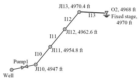
Figure 8‑6. Force main line

After these nodes are created, a set of force main pipes I10, I11, I12 and I13 are added between nodes JI10, JI11, JI12, JI13, and O2, respectively (refer to Figure 8‑6). The properties of these pipes are listed in Table 8‑5.

The final step is to add a pump link named PUMP1 between the nodes WELL and JI10. The pump curve (yet to be defined) associated with this pump is also named PUMP1, the initial status is Closed, and the startup depth is 5 ft while the shutoff depth is 2 ft. This means that the pump turns on when the water depth in the wet well reaches 5 ft and it shuts down when the depth drops to 2 ft.

Each pump added to an H2OMAP SWMM model is required to have a curve that defines how the pump’s discharge flow rate depends on the volume, depth or head added at its inlet (suction) side. This example will use a Type 3 pump curve where discharge varies inversely with the head (or lift) added by the pump between its inlet and outlet nodes. This type of curve provides the most realistic representation of how pumps actually behave and is usually available from the pump’s manufacturer. The head-discharge data that define the pump curve used here are listed in Table 8‑6. To add this curve to the model:

1. In the Attribute Browser, double-click on the field name “Pump Curve ID”. This will launch the Curve Editor.

2. Enter PUMP1 as the name of the curve and select 103: Pump Curve #3 (Head-Flow) as the curve type.

3. Enter the Head-Discharge data from Table 8‑6 into the grid on the form.

Table 8‑5. Properties of the force main line

Pipe ID	Shape	Inlet Node1	Length (ft)	Diameter (ft)	Rough. Coeff.	Inlet Offset (ft)	Outlet Offset (ft)
I10	Circular	JI10 (4947 ft)	500	2.0	0.016	0	0
I11	Circular	JI11 (4954.8 ft)	500	2.0	0.016	0	0
I12	Circular	JI12 (4962.6 ft)	500	2.0	0.016	0	0
I13	Circular	JI13 (4970.4 ft)	500	4.0	0.016	0	0
1 Number in parenthesis indicates the invert elevation of the node.

Table 8‑6. Pump curve data

Head (ft)	11	12	13	14	15	16	17	18	19	20	21	22	23	24
Discharge (cfs)	7.2	6.9	6.5	6.1	5.7	5.2	4.7	4.1	3.6	2.9	2.3	1.5	0.8	0

Dry Weather Flows

Wastewater flow from the sewersheds is added into the model using H2OMAP SWMM’s Node Inflow Editor tool (see the sidebar “Adding Dry Weather Flows into H2OMAP SWMM”). This example assumes that the individual Subcatchments in the model also represent the individual sewersheds. Only average daily dry weather inflows will be used to keep things simple.

Note: In reality, peak daily flows can be two to four times greater than the average. Therefore, if a more accurate analysis is required, a diurnal time pattern should be used to capture the full range of dry weather inflows. This, together with a continuous rainfall record, would allow one to simulate the dynamic performance of the system under all types of events.

Typical per capita domestic wastewater generation rates vary between 40 gpd (gallons per day) for apartments and 150 gpd for luxury residences and estates (Nicklow et al., 2004). ASCE (1992) defines a range of average per capita domestic loading rates between 50 gpd and 265 gpd. Based on these ranges and an estimate of 3 to 5 inhabitants per lot, an average domestic loading rate per lot of 300 gpd is assumed. In addition to the domestic rates, the discharge rates from the commercial areas in Subcatchments S5 and S6 also need to be included. These are estimated to be 2850 gpd in Subcatchment S5 and 8100 gpd in Subcatchment S5. The dry-weather flows for the Subcatchments are then computed as the sum of the domestic loading rate and the commercial rate. Table 8‑7 summarizes this computation, showing the number of residential lots in each Subcatchment (sewershed), the corresponding dry weather flows (in gpd and cfs) and the nodes that receive these inflows. Note that no dry weather flows are used in Subcatchments S6 and S7 because they contain no residential or commercial lots.

Table 8‑7. Summary of dry weather flows

Subcatchment	Node	Number of Residential Lots	Commercial Dry Weather Inflow	Dry Weather Inflow
				gpd	cfs
S1	J1	17	-	5100	0.008
S2	J2A	22	-	6600	0.010
S3	AUX3	10	-	3000	0.004
S4	J13_2	17	2850	5100+2850	0.0123
S5	J12_2	-	8100	8100	0.0125
S6	J11	-	-	0	0
S7	J10	-	-	0	0

Precipitation Data and Simulation Options

The 0.23 inches storm defined previously and both the 2-year and 10-year storms will be used to evaluate the performance of the combined sewer system. Dynamic Wave flow routing with a time step of 15 s, a 1 minute wet weather runoff time step, a 1 hr dry weather runoff time step, a 1 minute reporting time step and a total duration of 12 hours will be used in all the simulations. All the information for the model has been summarized in Table 8‑1 to Table 8‑7. The completed scenario is named ‘EX8-COMBINED_SEWERS’ (see ‘EX8-COMBINED_SEWERS’ ‘parent’ and ‘child’ scenarios in ‘H2OMAP SWMM Applications.HSM’).

8.4 Model Results

0.23 in. Storm

The model is first run for the 0.23 in. storm event. Viewing the Link Flow Summary of the resulting Status Report shows that there is no flow in any of the links that divert water from the combined sewers into the stream (W1_2, W2, W3, W4 and C6). Thus no CSOs occur for this size storm. Figure 8‑7 shows the flow through each channel of the stream. The only channel with any flow is C11 which receives only stormwater runoff (and no wastewater flow) from Subcatchment S7. Flows in any other of the stream’s conduits would imply that CSOs are occurring somewhere in the system.

Figure 8‑8 shows the flows through each section of the interceptor for the 0.23 in. storm. Note how the peak discharges and volumes increase in the downstream direction (from I1 to I9) as the different combined sewer pipes discharge into the interceptor through the flow regulators, as illustrated in Figure 8‑9. The latter figure shows that all the orifices and pipes that connect the combined sewers to the interceptor are contributing flows to the interceptor.

2-yr Storm

Results obtained for the 2-yr storm (with a volume of 1.0 in.) are now presented. Figure 8‑10 and Figure 8‑11 show the flows through the various stream and interceptor sections, respectively. Note that for this larger storm, flow occurs in all sections of the stream. The Link Flow Summary of the Status Report shows that CSOs occur and all the flow regulators start discharging flow into the stream once the capacity of diversion into the interceptor has been reached. The irregular fluctuations in flow through the interceptor seen in Figure 8‑11 are caused by fluctuations in the flow pumped into the force main at the pump station.

Figure 8‑7. Flow (Q) along sections of the stream for the 0.23 in. storm

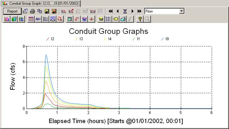
Figure 8‑8. Flow (Q) along sections of the interceptor for the 0.23 in. storm

Figure 8‑9. Flow (Q) diverted from each regulator to the interceptor for the 0.23 in. storm

Figure 8‑10. Flow (Q) along sections of the stream for the 2-yr storm

Figure 8‑11. Flow (Q) along the sections of the interceptor for the 2-yr storm

Figure 8‑12 and Figure 8‑13 compares the flows that are diverted into the interceptor and to the stream CSO for flow regulators R1 and R4. The interceptor diversions are from orifice Or1 and conduit I7, while the CSO discharges are from weirs W1 and W3. The regulators are able to convey the discharges into the interceptor for a while, but at a certain point the maximum capacity is reached and a CSO occurs. Note that the durations of CSOs are smaller than those of the discharges into the interceptor; however, the peak discharge is larger.

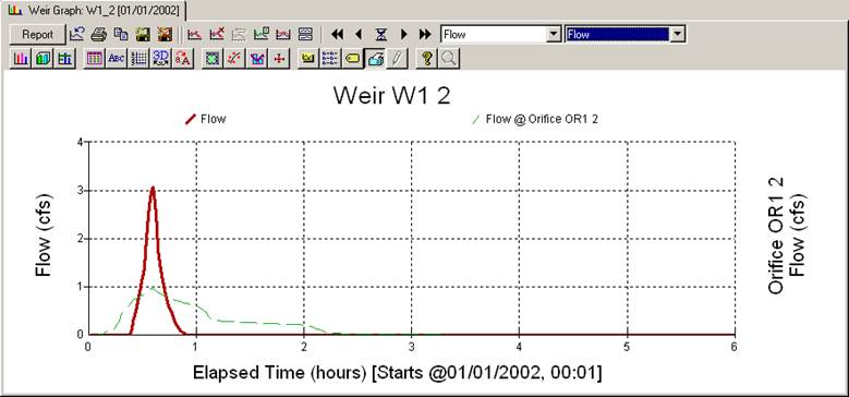
Figure 8‑12. Flows (Q) in regulator R1 for the 2-yr storm

Figure 8‑13. Flows (Q) in regulator R4 for the 2-yr storm

Pump Station Behavior

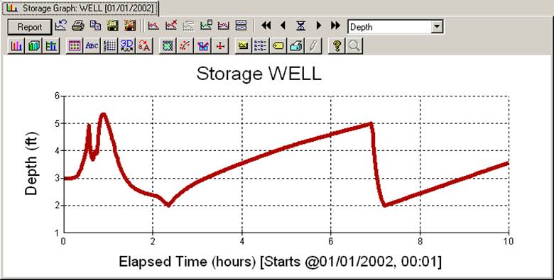
Figure 8‑14 shows how the pump in this combined system behaves under the 0.23 in. event. Part (a) of the figure plots the water depth in the pump’s wet well and part (b) shows the pump’s discharge flow rate. The startup and shutoff depths are shown with dashed lines. At the start of the simulation the water depth is 3 ft and the pump is initially off (Point 1). The pump turns on once the startup depth of 5 ft is reached (Point 2). Inflow to the pump station is large enough so that the pump continues working and the wet well water depth stays above the shutoff level. The water depth eventually reaches a maximum (Point 3) and then starts decreasing until reaching the 2 ft shutoff depth at which time the pump stops operating (Point 4). After the runoff flow ceases some 2+ hours into the simulation, only wastewater flows are received at the wet well, and the water depth increases slowly again until reaching the startup depth (Point 5); the pump turns on but rapidly stops when the shutoff depth is reached (Point 6). From hereafter pumped discharges fluctuate between the startup and shutoff limits.

Figure 8‑14. Pump behavior for the 0.23 in. storm: (a) wet well water depth, (b) pump flow

Overall Performance

Table 8‑8 compares the main results for the 0.23 in., 2-yr, and 10-yr storms. No CSOs occur for the 0.23 in. storm and all the wastewater flow is diverted into the interceptor. For the 2- and 10-yr storms, all the regulators are releasing discharges into the stream. Note how the occurrence of CSOs is reflected in the large increase in peak discharge at the receiving stream outfall O1. The peak discharge changes from 0.89 cfs for the 0.23 in. storm to 19.62 cfs for the 2-yr storm and 42.95 cfs for the 10-yr storm. Table 8‑8 also shows that the maximum discharge conveyed by the interceptor barely changes with the magnitude of the storm once all the regulators are discharging CSOs to the stream. The maximum water depth in the wet well is practically the same for the 2- and 10- year storm. This result clearly shows that flow regulators work in a way such that all the flows above the diversion capacity are directly discharged into the water body.

Table 8‑8. Summary of system performance for different storm events

System Performance Measure	0.23 in.	2-yr (1.0 in.)	10-yr (1.7 in.)
Max. wet well water depth (ft)	5.35	13.58	13.93
Max. interceptor pump flow (cfs)	7.2	7.2	7.2
Max. flow at stream outfall O1_2	0.89	19.62	42.95
Max. overflow at regulator R1 (cfs)	0	3.08	5.84
Max. overflow at regulator R2 (cfs)	0	5.06	5.30
Max. overflow at regulator R3 (cfs)	0	7.15	13.46
Max. overflow at regulator R4 (cfs)	0	9.22	13.08
Max. overflow at regulator R5 (cfs)	0	6.67	7.79

8.5 Summary

This example showed how to model a combined sewer system, composed of combined sewer pipes, flow regulators, a pump station and a force main line, within H2OMAP SWMM. The resulting model was used to determine the occurrence of Combined Sewer Overflows (CSOs) under different size storm events. The key points illustrated in this example were:

1. The main components of a combined sewer system model are pipes that carry both dry weather sanitary and wet weather runoff flows, flow regulators that divide flow between an interceptor pipe and a CSO outfall, and, if required, pump stations that carry interceptor flows to a treatment facility through a force main.

2. Continuous wastewater flows, which can vary periodically by time of day, day of week, and month of the year, are directly added into nodes associated with collector sewers that service individual sewersheds.

3. Flow regulators can be represented using a combination of pipes, orifices and weirs. The best way to model these regulators will depend on local conditions in the combined sewer system under analysis.

4. A pump station can be modeled using a storage unit node to represent the wet well that connects a pump link to the inlet node of a force main. The operation of the pump is defined through a pump curve and a set of wet well water levels that determine when the pump starts up and shuts down.

5. A force main line can be defined by using a set of pipes between junction nodes that are assigned a high surcharge depth so that flooding does not occur when the main pressurizes.

6. By examining a number of design storms (or by running a continuous simulation as described in the next example) one can determine the frequency at which combined sewer overflows will occur. In this particular example, the 0.23 in. storm produced no overflows while the 2-yr and 10-yr storms did. As shown from an analysis of the rainfall record for this site made in Example 9, roughly 1 in 4 storms is larger than 0.23 in. and would thus have the capability to result in a CSO.