Rainfall Dependent Inflow and Infiltration from the EPA SWMM 5 Hydrology Manual

7.1 Introduction

Rainfall dependent (or rainfall-derived) inflow and infiltration (RDII) are stormwater flows that enter sanitary or combined sewers due to "inflow" from direct connections of downspouts, sump pumps, foundation drains, etc. as well as "infiltration" of subsurface water through cracked pipes, leaky joints, poor manhole connections, etc. RDII can be a significant cause of sanitary sewer overflows (SSOs) of untreated wastewater into basements, streets and other properties, as well as receiving streams. It can also cause significant flow increases to wastewater treatment plants resulting in hydraulic overloading and disruption of plant processes.

SWMM treats RDII as a separate category of external inflows that enters the conveyance system at specific user-designated nodes. It is computed independently of the surface runoff, infiltration, snowmelt and groundwater processes described in previous chapters of this manual. RDII flow is added onto the other inflow categories (such as dry weather sanitary flow, overland runoff, and groundwater interflow) during each time step of a simulation. RDII calculations were added to version 4 of SWMM by C. Moore of CDM in 1993. This chapter describes how these RDII flows are computed from the precipitation records supplied to a SWMM data set.

Note: This section is an adaptation from the Storm Water Management Model Reference Manual Volume I – Hydrology By: Lewis Rossman U.S. Environmental Protection Agency Office of Research and Development National Risk Management Laboratory Cincinnati, OH 45268 National Risk Management Laboratory Office of Research and Development U.S. Environmental Protection Agency 26 Martin Luther King Drive Cincinnati, OH 45268 July 2015

7.2 Governing Equations

Figure 7-1 depicts the three major components of wet-weather wastewater flow within a sanitary sewer system (Vallabhaneni et al., 2007). These are base sanitary flow (BSF), groundwater infiltration(GWI), and RDII. BSF is the flow discharged to sanitary sewersby homes, businesses, institutions, and industrial water users throughout the normal course of a day. It exhibits a typical diurnal pattern, with higher flows during the morning and early evening hours and lower flows overnight. The average daily BSF remains more or less constant during the week, but can vary by both month and season.

GWI consists of groundwater that enters the collection system through cracked pipes, pipe joints and manhole walls during extended periods of time when water table levels are high, even in the absence of any rainfall. It is different from RDII because it does not occur as a direct response to a rainfallevent. GWI variesthroughout the year,with the highestrates in late winter and spring as groundwater levels rise, and the lowest rates (or no GWI at all) during late summer or after an extended dry period.

RDII is the flow that can be directlyattributed to a rainfall event.This flow is zero beforethe start of the event, increases during the event,and declines back to zero sometime after the event is over. The start of the RDII response may be delayed during the time it takes for surfaces to capture a portion of the initial rainfall and for soils to become saturated. If the event is small enough, then no RDII at all may be generated. The maximum volume of rainfallthat does not produce any RDII response is referred to as “initial abstraction” (Vallabhaneni et al., 2007).

Figure 7-1 Components of wet-weather wastewater flow.

Quantitative estimates of RDII are almost always derived from actual wastewater flow records as opposed to attempting to model the distributed set of small scale physical processes directly responsible for RDII. Methods for modeling RDII are reviewed by Bennet et al. (1999) and Lai (2008). SWMM uses the RTK unit hydrograph approach, which is among the most flexible and widely used RDII methods (Vallabhaneni et al., 2007). (The initials RTK stand for the three parameters that characterize the unit hydrographs used by the method.)

The RTK unit hydrograph method was first developed by CDM-Smith consultants in an RDII study for the East Bay Municipal Utility District in Oakland, CA (Giguere and Riek, 1983). It represents the response of a sewershed to a rainfall event through a series of up to three triangular

unit hydrographs. These unit hydrographs can be applied to any particular storm event to produce a resulting time history of RDII flow rates.

Figure 7-2 shows a single triangular unit hydrograph assumed to represent the RDII flow induced by one unit of rainfall over a unit of time. This unit hydrograph is characterized by the following parameters:

R: the fraction of rainfall volume that enters the sewer system and equals the volume under the hydrograph

T: the time from the onset of rainfall to the peak of the unit hydrograph K: the ratio of time to recession of the unit hydrograph to the time to peak Qpeak: peak flow (per unit area) on the unit hydrograph.

Figure 7-2 Example of an RDII triangular unit hydrograph.

Figure 7-3 shows how this single unit hydrograph would be applied to a storm that consists of three time periods of varying rainfall volume. The original unit hydrograph is replicated for each rainfall time period, with its origin offset by the time period and its ordinates multiplied by the rainfall volume for that period. The overall response to the storm is the hydrograph obtained by summing the ordinates of the volume-adjusted hydrographs at each time point. The volumetric RDII inflow into the conveyance system is the ordinate of the composite hydrograph multiplied by the contributing area of the affected sewershed. This process of adding together the rainfall- adjusted, time-shifted hydrographs is known as convolution (Chow et al, 1988) and is expressed mathematically as:

 

Figure 7-3 Application of a unit hydrograph to a storm event.

The ordinate value Uj for time period is determined from the shape parameters R, T,and K of the unit hydrograph as follows. One can write:

Because actual RDII hydrographs have complex shapes,three different hydrographs of increasing durations are typically used to represent the overall RDII unit response (Vallabhaneni et al., 2007). The first hydrograph modelsthe most rapidlyresponding inflow component usually caused by direct sources of inflow, and has a time to peak T of one to three hours. The second includes both rainfall-derived inflow and infiltration, and has a longer T value. The third represents infiltration that may continue long after the storm event has ended and has the longest T value. Figure 7-4 depicts how the three unit hydrographs are summed together to produce a total RDII hydrograph in response to a unit of rainfall over one unit of time. Equation 7-1 is still used to compute the overall RDII hydrograph to any given storm event, with a separate Qt computed for each of the three unit hydrographs. These are then added togetherto produce the total flow per unit area for time period t.

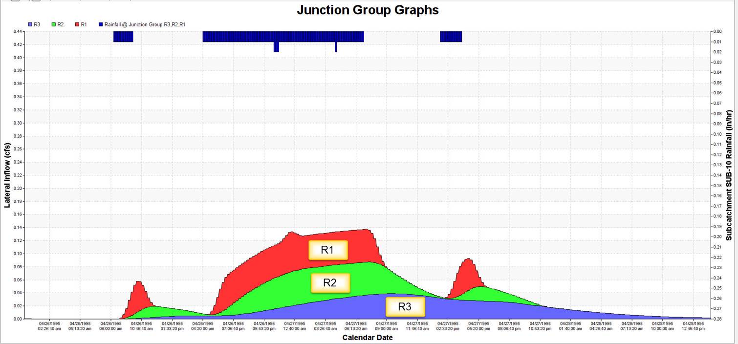
Figure 7-4 Use of three unit hydrographs to represent RDII (Vallabhaneni et al., 2007).

Not all storms will result in measurable inflow/infiltration. Just as with ordinary runoff, a certain initial volume of rainfall will be captured by surface ponding, interception by flat roofs and vegetation, and surface wetting and will not contribute to RDII. This phenomenon is represented in SWMM by three user-supplied “initial abstraction” (IA) parameters that accompany each RDII unit hydrograph. IAmax (in or mm) is the maximum depth of initial abstraction capacity available for the sewershed. IA0 (in or mm) is the amount of that capacity already used up at the start of the simulation. IAr (in/day or mm/day) is the rate at which capacity becomes available again during periods of no rainfall. During storm events, the volume of rainfall applied to the unit hydrograph convolution formula, Equation 7-1, is reduced by the amount of initial abstraction capacity

remaining. During dry periods, this capacity is regenerated based on the user-supplied recovery rate.

7.3 Computational Scheme

SWMM generates RDII inflows for specific nodes of a sewer system.Recall from Section1.2 that SWMM uses a networkof links and nodes to represent the conveyance portionof a drainage area. For RDII applications this network would be the sewer system (either sanitary or combined), the links are the sewer pipes and the nodes are points where pipes connect to one another (e.g., manholes or pipefittings).

It should be noted once again that RDII is computed independently from any surface runoff or groundwater flow generated from the subcatchments contained in a SWMM model.The sewershed that produces RDII flow for a specific sewer system node is not represented explicitly in SWMM and need not correspond to any of the runoffsubcatchments defined for the studyarea. In fact it is perfectly acceptable (and quite common for sanitary sewer systems) to conduct an RDII analysis without including any subcatchments in the model. In this case the model would consist of a set of Rain Gage objects (and their data sources), the node and link objects that make up the sewer network and sets of user-supplied time series that describe groundwater (GWI) and sanitary(BSF) flows.

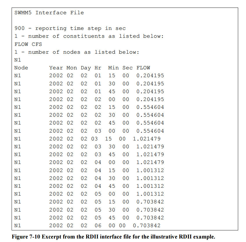
SWMM computes all RDII inflow time series prior to the start of a simulation and saves these inflow values to an interface file. Each line of the file contains, in chronological order, a node ID name, a date, a time of day, and the RDII inflow value for that node. Dates with no RDII inflows are not recorded. To compute the entries of this file the following quantities are assumed known for each node of the conveyance system node that receives RDII inflows:

The steps used to process a precipitation record against a set of unit hydrographs to produce a record of RDII inflows for a specific conveyance node are described in the sidebar shown below.

7.4 Parameter Estimates

To use SWMM’s RDII option a user must supply estimates of the three parameters (R, T, and K) that define each of three unit hydrographs for each node where RDII enters the sewer system.Each unit hydrograph can also have a set of initial abstraction parameters (Ia0, Iamax, and Iar). SWMM also allows one to specify different sets of unit hydrographs and initial abstraction parameters for differentmonths of the year. In addition, the area of the RDII contributing sewershed must also be specified.

R-T-K parameters are derived from site-specific flow monitoring data. There are no generalvalues that can be applied in the absence of actual field data. All of these parameters require that a continuous flow monitoring program be implemented at strategic points in the sewer system. As described in Vallabhaneni et al., 2007, estimating the RDII unit hydrograph parameters for a sewershed involves the following activities:

1. Identify the sewershed areas that are tributary to the flow monitor (see Figure 7-5).

2. Extract the RDII portion of the recorded flow at the monitoring station during a wet weather event (see Figure 7-6).

3. Estimate the R-T-K values for each of three unit hydrographs whose resultant hydrograph best matches the RDII flow extracted from the flow record (see Figure 7-7).

7.5 Numerical Example

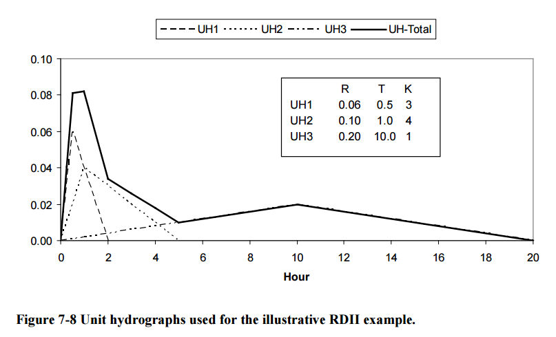
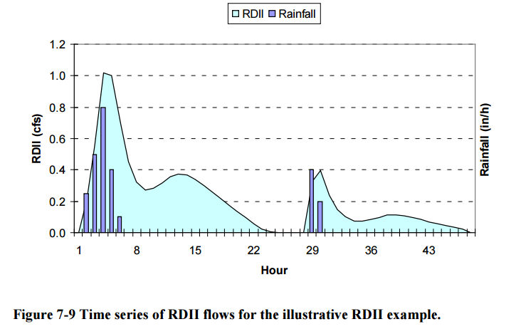
A simple example illustrates how SWMM constructs an RDII interface file for use within a hydraulic simulation. Assume there is a single rain gage whose rainfall time series is shown in Table 7-1. Note that the recording intervalis 1 hour, and that there are two eventsseparated by 22 hours. SWMM will use data from this gage to construct a time series of RDII flows for a node named N1 in the conveyance systemthat services an area of 10 acres.There is a single group of 3 unit hydrographs used to derive RDII from the rain gage data. The shapes and parameters of the unit hydrographs (UH1, UH2, and UH3) are shown in Figure 7-8. Note that the R-values of this set of unit hydrographs sum to 0.36, implying that 36 percent of total rainfall volume winds up as RDII. To keep things simple, initial abstraction is not considered in this example.

Table 7-1 Rainfall time series for the illustrative RDII example

Hour	Rainfall (inches)
0:00	0.0
1:00	0.25
2:00	0.5
3:00	0.8
4:00	0.4
5:00	0.1
6:00	0.0
27:00	0.0
28:00	0.4
29:00	0.2
30:00	0.0

The resulting RDII flows are depicted in Figure 7-9. SWMM places these flows into an RDII interface file, a portion of which is displayed in Figure 7-10. This file is accessed during the flow routing portion of a SWMM run to add RDII inflow into node N1 at each time step of the routing process.

N1
Node N1	Year Mon Day Hr 2002 02 02 01				Min Sec FLOW 15 00 0.204195
N1	2002 02	02	01		30		00		0.204195
N1	2002 02	02	01		45		00		0.204195
N1	2002 02	02	02		00		00		0.204195
N1	2002 02	02	02		15		00		0.554604
N1	2002 02	02	02		30		00		0.554604
N1	2002 02	02	02		45		00		0.554604
N1	2002 02	02	03		00		00		0.554604
N1	2002 02	02 03		15		00		1.021479
N1	2002 02	02	03		30		00		1.021479
N1	2002 02	02	03		45		00		1.021479
N1	2002 02	02	04		00		00		1.021479
N1	2002 02	02	04		15		00		1.001312
N1	2002 02	02	04		30		00		1.001312
N1	2002 02	02	04		45		00		1.001312
N1	2002 02	02	05		00		00		1.001312
N1	2002 02	02	05		15		00		0.703842
N1	2002 02	02	05		30		00		0.703842
N1	2002 02	02	05		45		00		0.703842
N1	2002 02	02	06		00 00			0.703842