Stormwater Modelling in InfoSewer and H2OMap Sewer
Steady-state analysis and design of storm sewers is usually accomplished under worst (i.e., peak) runoff conditions to test transporting capacity of the network without causing major flooding or overflows. The Rational method is the most widely used technique for estimation of peak flow from urban and rural drainage basins, and is the method used by InfoSewerH20Map Sewer during steady-state analysis and design .
The Rational method is based on the premise that if rainfall occurs over a watershed at a constant intensity for a period of time that is sufficiently long to produce steady state runoff at a desired design point, such as at manhole locations, then the peak flow rate will be proportional to the product of rainfall intensity and watershed area. Peak runoff is assumed to occur when all locations in the subwatersheds draining to the point contribute flow. The rainfall intensity is considered constant over a duration commonly known as time of concentration.
Mathematically, the Rational method is expressed as:
![]()
where Q = peak runoff rate (flow unit)
C = runoff coefficient (unitless)
i = rainfall intensity (intensity unit)
A = watershed area (area unit).
Time of concentration for a loading manhole is calculated as the sum of overland flow travel time and pipe flow travel time. Overland flow travel time is estimated using Kirpich's equation as shown below.
![]()
where to = overland flow travel time for a subwatershed (in minutes)
L = length of flow path from the remotest spot in the subwatershed (in feet)
S = average slope of the subwatershed
Detailed description of the theoretical aspect of the Rational method is given in InfoSewerH20Map Sewer Theory section.
InfoSewerH20Map Sewer could be used for modeling of sanitary sewer systems, storm sewer systems, or combined sewer systems. A user interested in performing steady state simulation of storm and/or combined sewer systems needs to provide the following data for every loading manhole in addition to the data required for modeling of sanitary sewers.
· Runoff coefficient (C)
· Length of flow path from the remotest spot in the subwatershed (L)
· Average slope of the subwatershed (S)
· Area of the subwatershed (A)
If US Customary units are used, area and length should be given in acres and in feet , respectively. If SI units are used, area should be in square meters, and length should be in meters.
These manhole data could be supplied to the model either through the attribute browser or by using the manhole hydraulic/hydrologic data base table.
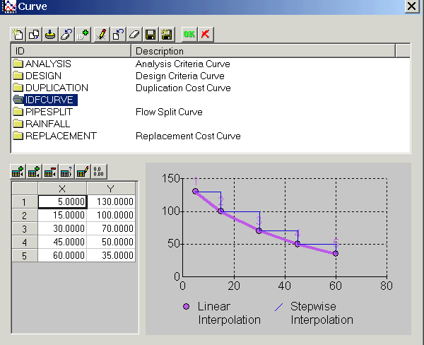
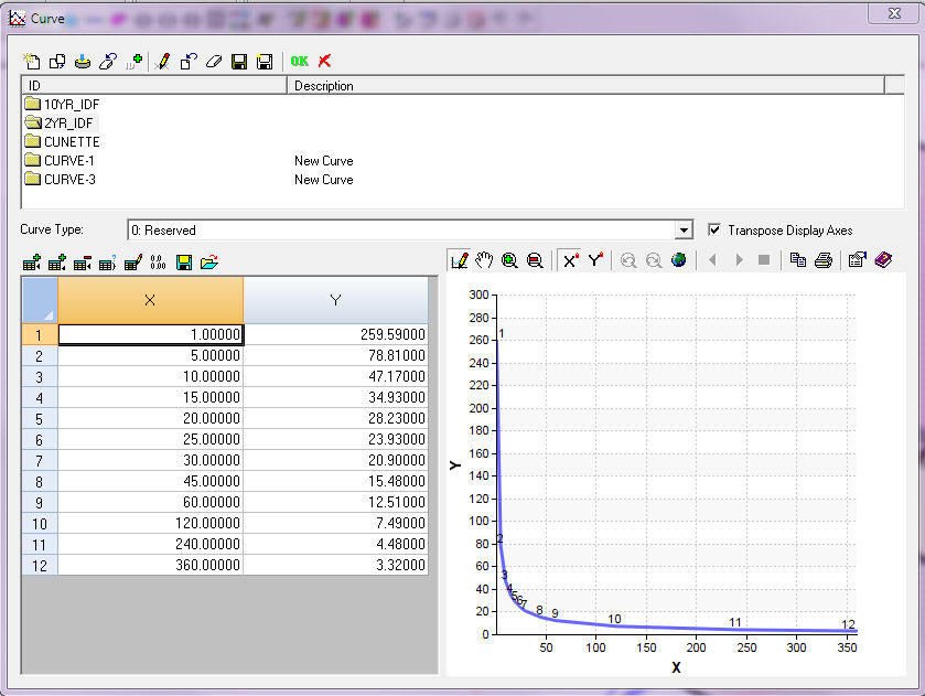
In addition to the above mentioned data, the user has to provide an Intensity-Duration-Frequency curve of the watershed for a desired return period. An IDF data is accepted in the form of a curve, where the y-axis represents rainfall intensity and the x-axis represents rainfall duration. A typical IDF curve is shown below. The model accepts rainfall intensity in any of the following units: inches/hour, mm/hour, inches/minute, or mm/minute. Rainfall duration could be in second, in minute, or in hour.
In order to avoid unreasonably low storm duration and unreasonably high rainfall intensities, InfoSewerH20Map SewerPro allows the user to specify a minimum time of concentration to be used by the Rational method. The model uses the maximum of the user specified minimum time of concentration and an internally calculated time of concentration. The default value used by the model for the minimum time of concentration is 10 minutes.
To supply an IDF curve and its intensity and duration units, and the minimum time of concentration data, the modeler needs to follow the following procedure.
· Go to the simulation options dialog box shown below either from the control center or using the run manager.
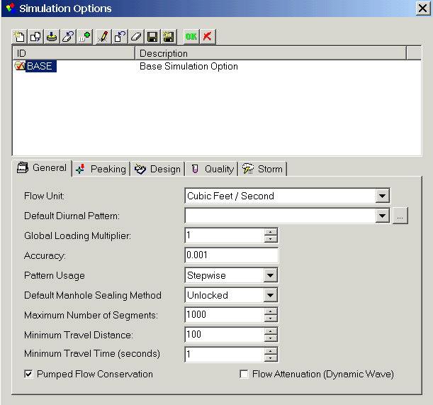
· Click on ![]() icon . This initiates the following storm dialog box.
icon . This initiates the following storm dialog box.
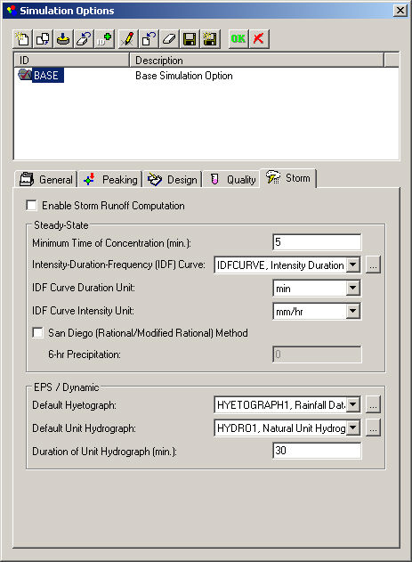
· Check ![]() option to activate storm simulation.
option to activate storm simulation.
· Supply data for minimum time of concentration, IDF Curve, and duration and intensity units of the IDF curve.
For the IDF Curve, the model accepts rainfall intensity in any of the following units: inches/hour, mm/hour, inches/minute, or mm/minute. Rainfall duration could be in second, in minute, or in hour.
The user has to provide an Intensity-Duration-Frequency curve of the watershed for a desired return period. An IDF data is accepted in the form of a curve, where the y-axis represents rainfall intensity and the x-axis represents rainfall duration.
In order to avoid unreasonably low storm duration and unreasonably high rainfall intensities, H2OMAP Sewer Pro allows the user to specify a minimum time of concentration to be used by the Rational method. The model uses the maximum of the user specified minimum time of concentration and an internally calculated time of concentration. The default value used by the model for the minimum time of concentration is 10 minutes.
· San Diego Rational/Modified Rational Method uses the San Diego County rational method and modified rational method to calculate peak storm flow for storm drains.
· 6-hr Precipitation is the six hour duration rainfall depth for the design return period.
· Save the changes and close the dialog box.
· If the loading manhole data required for steady state simulation of stormwater, as described above, are already provided, the desired simulation (i.e., steady state analysis or steady state design) could be performed from the run manager.
· If the type of the simulation is steady state analysis, the model reports peak storm load for every loading manhole and pipe in the collection system. Results are available from the attribute browser.
· If the type of the simulation is steady state analysis, the model reports peak storm load for every loading manhole and pipe in the collection system. Results are available from the attribute browser.
Infiltration 
Both infiltration and inflow affect the operation of a sanitary sewer system and pumping, treatment, and overflow regulators facilities. The infiltration load in the pipe is listed as an external load into the upstream manhole. The load is a point load and is not distributed over the length of the link. Infiltration occurs in gravity pipes while inflow occurs at manholes and wet wells. Infiltration loads refer to the volume of groundwater entering the sewer system from the soil through defective joints, broken or cracked pipes, improper connections, or manhole walls. It can be derived by subtracting base flow from total metered flow during dry weather or by compiling flow isolation measurements. Infiltration can be defined as proportional to the pipe length; proportional to the pipe length and to the pipe diameter; proportional to the pipe surface area (pipe length multiplied by its perimeter); proportional to the number of defects in the pipe (count-based); or as a pattern load/hydrograph (flow vs. time) as shown below:
Creating Infiltration
A gravity main needs to be first selected by the user. The user can then click on the Infiltration icon located on the Attribute Browser to launch the following dialog box. The different methods to assign infiltration is explained as below:
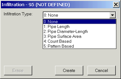
· 1: Pipe Length: The infiltration is defined as an infiltration rate per unit of pipe length. The amount of infiltration is proportional to the pipe length. If the pipe is 200 feet long and I enter a 1 then the infiltration flow is 200 MGD which mean the infiltration rate unit is mgd/foot/day
· 2: Pipe Diameter-Length: The infiltration is defined by an infiltration rate per unit of pipe diameter times pipe length. The amount of infiltration is proportional to the pipe length and to the pipe diameter.
· 3: Pipe Surface Area: The infiltration is specified by an infiltration rate per unit of pipe surface area. The pipe surface area is calculated as its length multiplied by its full perimeter. The amount of infiltration is proportional to the pipe length and to the pipe diameter.
· 4: Count-Based: The infiltration is specified by an infiltration unit count value (for example, this may be the number of defects in the pipe) and the infiltration rate per unit of count.
· 5: Pattern-Based: The infiltration is specified by an infiltration rate and a pattern. A pattern consists of a collection of multipliers (multiplication factors) that are applied to a base infiltration rate to allow it to vary over time during an EPS/Dynamic simulations.
Infiltration Load
The pipe infiltration enters the network as a load at the upstream node of the link. The infiltration load in the pipe is listed as an external load into the upstream manhole. The load is a point load and is not distributed over the length of the link.
RDII or Tri Triangular Unit Hydrograph
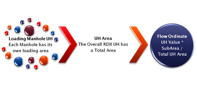
The RDII or Rainfall Dependent Infiltration Inflow method in InfoSewer is similar to the RDII or RTK method in InfoSWMM and InfoWorks ICM but with some differences. The RTK data for triangles 1, 2 and 3 are defined in the Unit Hydrograph but instead of individual R values, the overall R is set and the Percent R1, R2 and R3 are defined based on the total R. R3 is calculated internally as 100 – R1 – R2. Each loading manhole with RDII flow has a total area, a hyetograph and a Unit Hydrograph. The hyetograph has to be set at multiples of the unit hydrograph, so you can define the time or X columns with integers and then use the Block Edit command to change X to minutes by multiplying by the Unit Hydrograph time (Figure 1). You can use only one component if you set R1 or R2 to 100 percent or R3 to 100 percent by setting R1 and R2 to 0 percent (Figure 2). The overall area of the Unit Hydrograph is divided amongst the loading manhole using the Subbasin Area (Figure 3). The storm flows generated can be viewed using a Group Graph (Figure 4) and the area of the loading manholes has a relationship to to the total area of the defined unit hydrograph (Figure 5).
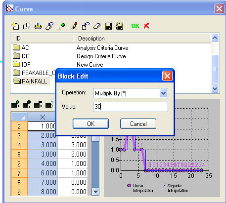
Figure 1. Hyetograph Curve for the RDII Unit Hydrograph
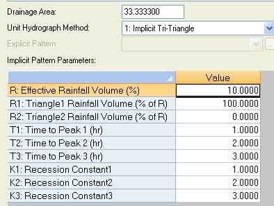
Figure 2. The Unit Hydrograph is defined for various values of R, R1, R2, T1, T2, T3, K1, K2 and K3
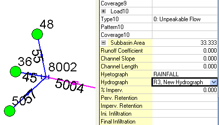
Figure 3. The-Unit-Hydrograph-and-Hyetograph-are-tied-to-a-particular-loading-manhole-using-a-Subbasin-Area
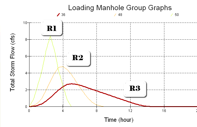
Figure 4. The Unit Hydrographs that are generated can be viewed using a Group loading Manhole Graph. The R1, R2 and R3 have only one triangle
Intensity-Duration-Frequency Curve
The relationship between rainfall intensity, rainfall duration, and frequency of occurrence of storm events is often presented for a certain region in the form of an Intensity-Duration-Frequency Curve, commonly referred to as an IDF curve. A sample IDF curve is given below for return periods of 5, 10, and 50 years.InfoSewerH20Map Sewer Pro calculates the rainfall intensity used by the Rational method based on a user-specified IDF curve. The user should provide an IDF curve for a desired return period. The model derives rainfall intensity from the IDF curve corresponding to the duration equal to the time of concentration calculated for the manhole following the techniques described above.


Sewer IDF Curve Table in the Atrribute Browser in USA Units
An Example IDF Curve from InfoSWMM in SI Units