2D Flood Routing Basics in InfoSWMM 2D

This methodology describes the basics of 2D overland flood routing with the InfoSWMM 2D extension to InfoSWMM.

• Glossary
• Introduction
• The 2D Zone
• Creating the 2D Zone
• Connecting the 1D Network to the 2D Zone
• Reviewing 2D Simulation Output
• Visualizing 2D Simulation Output
• References
• 2D Hydraulic Theory

Glossary

Term	Definition
2D Zone (2D Simulation Polygon)	Area within which the mesh is created.
Mesh Zone	Optional area within which the size of the mesh triangles can be changed from the default. Mesh zones exist within 2D zones.
Roughness Zone	Optional area within which the surface roughness can be changed from the default. Roughness zones exist within 2D zones.
Mesh	Series of joined triangles which form the 2D surface, created within the 2D Simulation Polygon.
Shewchuk Triangle	Method of triangulation used to form the mesh (See Reference 1).
Boundary Polyline	Optional lines used to change the boundary properties along a specific segment of the 2D Simulation Polygon
Porous Polygon	Optional polygons which allow you to control how much flow passes through (if any).
Porous Wall	Optional lines which.
Break Line	Optional lines used in the creation of the mesh.

Introduction

To be able to use this functionality, you must have InfoSWMM 2D installed and licensed when using it with InfoSWMM.

The InfoSWMM 2D extension works in combination with the InfoSWMM one dimensional calculation engine. Once manholes start to flood, the floodwater flows across a two dimensional zone representing the surface of the sub-catchment. Once flow reaches another manhole, it re-enters the 1D system and is controlled by the InfoSWMM calculation engine.

Top of Page

The 2D Zone

The 2D zone, alternatively described as a mesh, consists of a series of contiguous triangles, whose shared boundaries cover the catchment surface. The height of each point on each triangle is derived from a ground model GRID or TIN.

It is significant that the 2D zones are meshed, where the size and orientation of the triangles can be varied, rather than a grid, where the layout is fixed. Meshes allow more detail and complexity in locations only where it is needed.

Triangles are derived using the Shewchuk triangulation method (Reference 1).

Each 2D zone must include a boundary and the characteristics of the triangles within the zone must be defined. The creation of a 2D zone is described below. A 2D zone can include the following elements:

• Porous Wall Polylines are polylines use to impede or prevent flow through them. A common application of these features are to model fences.
• Porous Polygons are polygons used to impede or prevent flow through them. A common application of these features are to model buildings.
• Break Polylines are lines along which mesh triangle boundaries must be created. These can be used to define the top of a ridge or the low point in a channel.
• Boundary Polylines are optional lines (but must be created coincident to 2D Simulation Polygon boundaries) and are used to alter boundary properties along the line.
• Mesh Polygons are polygons within the 2D Simulation Polygons (2D zones) where the triangles have different maximum triangle area. They are most commonly used to define smaller triangles in areas of greater complexity.
• Initial Conditions (IC) Polygons are polygons within the 2D Simulation Polygons (2D zones) where the area has specific initial depth and velocity conditions.
• Roughness Polygons are polygons within the 2D Simulation Polygons (2D zones) where the area has specific Manning's roughness that differs from the roughness value of the 2D Simulation Polygon.
• 2D Simulation Polygons are polygons that define the outer boundary of a 2D zone. 2D Mesh will only be generated within these boundaries and 2D simulation will also happen only within these boundaries.

Each object can be either created within InfoSWMM 2D, or created in a GIS and then imported using the provided import tools.

2D zone triangles (2D Mesh) can be created once all the objects and the ground model have been prepared.

The interaction with the below ground system whereby water floods from the manholes on to the 2D zone and then possibly back into the manholes is also described below.

Top of Page

Creating The 2D Zone

Step 1 - Add ground surface data to the map

• Click the ArcMap Add Data button
• Browse to the location of your ground surface layer. Many different formats are supported.

Step 2 - Create 2D Simulation Polygons

1. Click the Create 2D Polygon button from the InfoSWMM 2D Toolbar
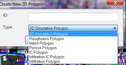
2. Digitize the polygon by clicking in the ArcMap Drawing Area on the first vertex then click additional vertices as needed. Double-click on the last vertex to complete the polygon.
3. Give the polygon a unique ID (and optional description if desired). Choose '2D Simulation Polygon' as the Type.
   
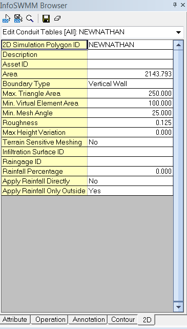
4. Notice that the attributes of the polygon you just created are shown in the 2D Tab in the Attribute Browser.
   
5. Adjust the attributes as needed to suit your modeling situation. For a description of attributes, click 2D Simulation Polygon.

Step 3 - Create Optional 2D Zone Modification Objects as Needed

Determine which 2D Zone modification objects you will need to correctly model the characteristics of your ground surface and any flow obstructions in the 2D Zone. The available modification objects are:

• 2D Boundary
• 2D Break Polyline
• 2D Initial Conditions Polygon
• 2D Mesh Polygon
• 2D Porous Polygon
• 2D Porous Wall Polyline
• 2D Roughness Polygon

Step 4 - Add 2D Point Source Objects

1. If there are any sources of additional flow onto the ground surface such as water springs or artesian wells, add them to the 2D simulation by adding 2D Point Source.

Step 5 - Create Initial Conditions Settings

It is often helpful to set up initial conditions for the 2D Zone. This is done by creating Initial Condition Settings and assigning them to 2D Simulation Polygons and IC Polygons. Initial Conditions associated with IC Polygons will override Initial Conditions associated with the 2D Simulation Polygon at that location.

1. Click Initial Conditions from the InfoSWMM 2D menu.
   
2. Click the New button to create a new Initial Condition.
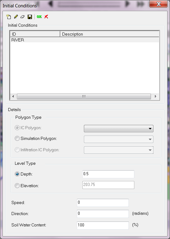
3. Choose which IC Polygon or 2D Simulation Polygon that the Initial Conditions should apply to.
4. Choose whether the initial level is specified by Depth or Elevation and enter the appropriate value.
5. Enter initial velocity information as Velocity and Direction (measured counter-clockwise from due East)
6. Repeat steps 2-5 for each IC Polygon or 2D Simulation Polygon that you wish to create Initial Conditions for.

Top of Page

Connecting the 1D Network to the 2D Zone

It is very simple to connect the 2D Zone to the 1D underground network and to enable the 2D simulation.

Step 1 - Set 2D Options

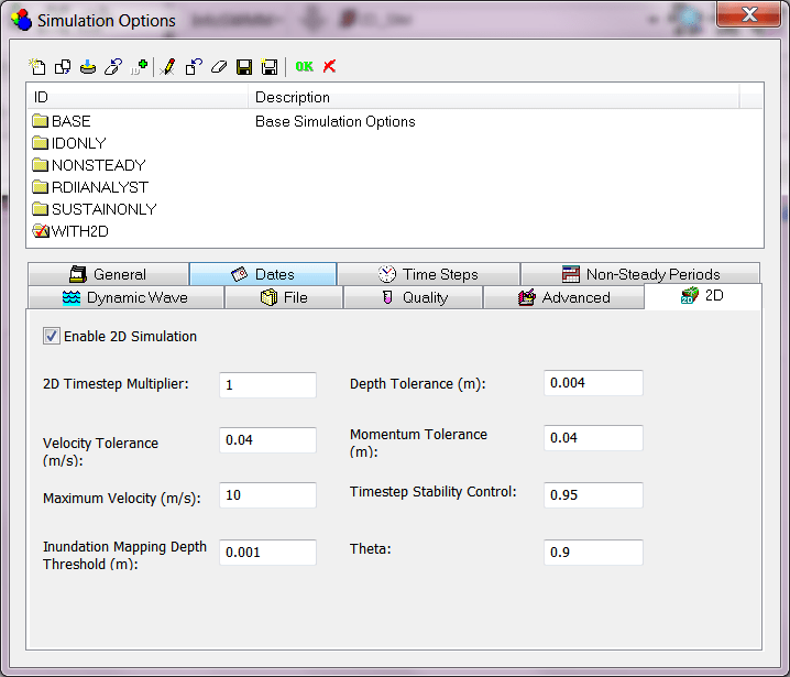
1. Open the Simulation Options that are associated with the scenario you wish to apply the 2D Zone to and select the 2D tab.
   
2. Select the 'Enable 2D Simulation' option and set the 2D simulation parameters. For a description of parameters, click 2D Simulation Options.
3. Set Dynamic Wave as the Routing Model on the General tab of the InfoSWMM Simulation Options.

Step 2 - Set Up 1D Junctions to Interact with 2D Zone

The 1D (underground) network and 2D (overland) Zone interact through the rim of 1D junctions. The junctions that are to interact with the 2D Zone need to be enabled and their rim elevations aligned with the 2D Mesh.

1. To enable a 1D junction to pass flow back and forth to the 2D Zone, select 2D as the Flood Type in the InfoSWMM Atrribute Browser.
   
2. Enter a Flood Discharge Coefficient. The orifice equation governs flow into and out of the rim of the junction.Q = C

   FDA(2gH)1/2where:

   Q = flow into or out of junction to/from 2D simulation

   CFD = Flood Discharge Coefficient. The Flood Discharge Coefficient combines the typical orifice coefficient (approximately 0.6) with an orifice area reduction factor (or porosity factor) that reduces the manhole surface area to an effective orifice area representing the small holes in a manhole cover or a slightly open or lifted cover. Example: An orifice coefficient of 0.60 is assumed and the effective flow area (i.e. effective orifice area) is 10% of the manhole surface area (12.56 ft2 for a 4 ft diameter manhole) then the Flood Discharge Coefficient is CFD = 0.60 X 0.1 = 0.06. Some studies have been done and papers have been written on the subject (see Reference 3).

   A = Area of junction (determined by the Minimum Surface Area parameter)

   H = Height difference across the 'orifice'

Step 3 - Align Junction Rim with 2D Mesh Elevations

It is important that the manhole ground levels match the height of the ground model at the relevant location. Otherwise flow could spill on to the mesh either earlier or later than it reaching the manhole ground level. Either:

1. Manually adjust junction rim elevations (or max depths) to match the ground elevation model you are using at that location. You can use the ArcMap Identify tool to check the elevation of the ground model at that location and adjust the rim elevation in the InfoSWMM Atrribute Browser for that junction. Or...
2. Alternatively, you can add all of the 2D junctions to a Domain and use the Elevation Extraction tool to extract rim elevations directly from the ground model you are using (limit the scope of elevation extraction to the Domain of 2D junctions).

Top of Page

Reviewing 2D Simulation Output

Once the model has been successfully simulated using the Run Manager, you can review the 2D simulation output. You can review the output by creating any of three types of output objects. The following output objects are available:

2D Result Point - This gives results at a specific point in a 2D Zone. The available output results for a point are:

• Depth - Depth of water above ground surface
• Direction - Direction of flow (angle in radians counter-clockwise from due East)
• Elevation - Water surface elevation (i.e. ground surface elevation plus Depth)
• Froude Number
  • Velocity
  • Unit Flow - Flow per unit length (i.e. Depth x Velocity)

2D Result Line - This gives results along a specific line in the 2D Zone. The available output results for a line are:

• Flow (through results analysis line) - The Flow through results analysis line result is calculated by summing the flows across each line segment.
• Maximum Depth (along results analysis line) - The maximum of the depth values of the 2D mesh elements intersected by the results analysis line.
• Maximum Speed (normal to results analysis line) - For each 2D mesh element that the 2D Results Line intersect, the maximum of the calculated values is reported as the maximum velocity. This is an absolute value.

2D Result Polygon - This gives results within a specific polygonal region in the 2D Zone. The available output results for a polygon are:

• Flow (through results analysis polygon boundary) - For each 2D mesh element that the 2D Results Polygon intersects, the Flow through results analysis polygon boundary result is calculated by summing the flows across each boundary segment. Flow directed into the polygon is counted positive and flow directed out of the polygon is counted negative.
• Maximum Depth (inside results analysis polygon) - The maximum of the depth values of the 2D mesh elements inside the results analysis polygon boundary. Only mesh elements with element centroid within the polygon boundary are included.
• Maximum Velocity (inside results analysis polygon) - The maximum of the velocity values of the 2D mesh elements inside the results analysis polygon boundary. Only mesh elements with element centroid within the polygon boundary are included.
• Volume (enclosed by results analysis polygon) - The volume enclosed by results analysis polygon result is calculated as the sum of water depth x element area of all 2D mesh elements within the polygon boundary. Only mesh elements with element centroid within the polygon boundary are included in the calculation.

To find out how to create a 2D Results Point, Click Create a 2D Results Point

To find out how to create a 2D Results Polyline, Click Create_a_2D_Results_Polyline

To find out how to create a 2D Results Polygon, Click Create_a_2D_Results_Polygon

Top of Page

Visualizing 2D Simulation Output

Once the model has been successfully simulated using the Run Manager, you can review the 2D simulation output. 2D Simulation results can be visualized in plan view (i.e. 2D view in the ArcMap Drawing Area window) or 3D view. Note: ArcGIS 3D Analyst extension must be installed and licensed to allow 3D view.

Visualize Output in 2D View

1. Click the 2D Map Display button from the InfoSWMM 2D Toolbar
2. Choose map display parameters according to the directions in 2D Map Display
3. The map coloration and velocity arrows will reflect output at the current time step. To change the visualization time step, use the InfoSWMM time slider
4. Optionally, you can use the InfoSWMM Animation Editor to create animations that show 1D network and 2D Zone simulation output.

Visualize Output in 3D View (ArcGIS 3D Analyst required)

1. Click the 3D View button from the InfoSWMM 2D Toolbar
2. Enter the 3D View parameters according to directions in 2D Show Results In 3D
3. Background and 1D layers can be displayed and buildings (2D Porous Polygon) can be extruded for a more realistic look
4. Water depth across the 2D zone can also be visualized within this view.

Top of Page

References

• Shewchuk, Jonathan Richard. A Two-Dimensional Quality Mesh Generator and Delaunay Triangulator. Computer Science Division, University of California at Berkeley, Berkeley, California 94720-1776. http://www.cs.cmu.edu/~quake/triangle.html
• Francisco Alcrudo, Pilar Garcia-Navarro. A high-resolution Godunov-type scheme in finite volumes for the 2D shallow-water equations. Departmento de Ciencia y Technologia de Materiales y Fluidos, Facultad de Ciencias, Universidad de Zaragoza, Zaragoza 50009, Spain. Presented in International Journal for Numerical Methods in Fluids, Volume 16, Issue 6.
• Z. Mustaffa, N. Rajaratnam, David Z. Zhu. An Experimental Study of Flow Into Orifices and Grating Inlets on Streets. Can. J. Civ. Eng. 33: 837-845 (2006)

Top of Page

Privileged and Confidential Communication: This electronic mail communication and any documents included hereto may contain confidential and privileged material for the sole use of the intended recipient(s) named above. If you are not the intended recipient (or authorized to receive for the recipient) of this message, any review, use, distribution or disclosure by you or others is strictly prohibited. Please contact the sender by reply email and delete and/or destroy the accompanying message.