EPA/600/R-16/093 | July 2016 | www.epa.gov/water-researchUnited States Enviromental Protection AgencyStorm Water Management Model Reference ManualVolume III – Water QualityOffice of Research and Development
Water Supply and Water Resources Division
EPA/600/R-16/093
July 2016
Storm Water Management Model Reference Manual
Volume III – Water Quality
By:
Lewis A. Rossman
Office of Research and Development National Risk Management Laboratory
Cincinnati, OH 45268
and Wayne C. Huber
School of Civil and Construction Engineering
Oregon State University Corvallis, OR 97331
National Risk Management Laboratory Office of Research and Development
U.S. Environmental Protection Agency 26 Martin Luther King Drive
Cincinnati, OH 45268
July 2016
Disclaimer
The information in this document has been funded wholly or in part by the
U.S. Environmental Protection Agency (EPA). It has been subjected to the
Agency’s peer and administrative review, and has been approved for
publication as an EPA document. Mention of trade names or commercial
products does not constitute endorsement or recommendation for use.
Although a reasonable effort has been made to assure that the results
obtained are correct, the computer programs described in this manual are
experimental. Therefore the author and the U.S. Environmental Protection
Agency are not responsible and assume no liability whatsoever for any
results or any use made of the results obtained from these programs, nor for
any damages or litigation that result from the use of these programs for any
purpose.
Abstract
SWMM is a dynamic rainfall-runoff simulation model used for single event or
long-term (continuous) simulation of runoff quantity and quality from
primarily urban areas. The runoff component of SWMM operates on a collection
of subcatchment areas that receive precipitation and generate runoff and
pollutant loads. The routing portion of SWMM transports this runoff through
a system of pipes, channels, storage/treatment devices, pumps, and
regulators. SWMM tracks the quantity and quality of runoff generated within
each subcatchment, and the flow rate, flow depth, and quality of water in
each pipe and channel during a simulation period comprised of multiple time
steps. The reference manual for this edition of SWMM is comprised of three
volumes. Volume I describes SWMM’s hydrologic models, Volume II its
hydraulic models, and Volume III its water quality and low impact
development models.
Acknowledgements
This report was written by Lewis A. Rossman, Environmental Scientist
Emeritus, U.S. Environmental Protection Agency, Cincinnati, OH and Wayne C.
Huber, Professor Emeritus, School of Civil and Construction Engineering,
Oregon State University, Corvallis, OR.
The authors would like to acknowledge the contributions made by the
following individuals to previous versions of SWMM that we drew heavily upon
in writing this report: John Aldrich, Douglas Ammon, Carl W. Chen, Brett
Cunningham, Robert Dickinson, James Heaney, Wayne Huber, Miguel Medina,
Russell Mein, Charles Moore, Stephan Nix, Alan Peltz, Don Polmann, Larry
Roesner, Lewis Rossman, Charles Rowney, and Robert Shubinsky. Finally, we
wish to thank Lewis Rossman, Wayne Huber, Thomas Barnwell (US EPA retired),
Richard Field (US EPA retired), Harry Torno (US EPA retired) and William
James (University of Guelph) for their continuing efforts to support and
maintain the program over the past several decades.
Portions of this document were prepared under Purchase Order 2C-R095-NAEX to
Oregon State University.
Table of Contents
APWA American Public Works Association ASCE American Society of Civil
Engineers BMP Best Management Practice
BOD Biochemical Oxygen Demand
BOD5 Five-Day Biochemical Oxygen Demand C Carbon
Cd Cadmium
COD Chemical Oxygen Demand
COV Coefficient of Variation
Cr Chromium
CSO Combined Sewer Overflow
Cu Copper
DCIA Directly Connected Impervious Area DD Dust and Dirt
DWF Dry Weather Flow
EMC Event Mean Concentration
EPA Environmental Protection Agency
ET Evapotranspiration
Fe Iron
GI Green Infrastructure
IMP Integrated Management Practice
JTU Jackson Turbidity Units
LID Low Impact Development
Mn Manganese
MPN Most Probable Number MTBE Methyl Tertiary Butyl Ether
NADP National Atmospheric Deposition Program NH3-N Ammonia Nitrogen
NH4 Ammonium
Ni Nickel
NO2 Nitrite
NO3 Nitrate
NPDES National Pollution Discharge Elimination System NURP National Urban
Runoff Program
PAH Polycyclic Aromatic Hydrocarbons Pb Lead
PCU Platinum-Cobalt Units
PO4 Phosphate
RDII Rainfall Dependent Inflow and Infiltration Sr Strontium
SCM Stormwater Control Measure
SUDS Sustainable Urban Drainage Systems SWMM Storm Water Management Model
TDS Total Dissolved Solids
TKN Total Kjeldahl Nitrogen
TN Total Nitrogen
TOC Total Organic Carbon
TP Total Phosphorus
TPH Total Petroleum Hydrocarbons
TSS Total Suspended Solids
UK United Kingdom
USGS United States Geological Survey VOC Volatile Organic Carbon
WPCF Water Pollution Control Federation WWTP Waste Water Treatment Plant
Zn Zinc
Chapter 1 – Overview
Introduction
Urban runoff quantity and quality constitute problems of both a historical
and current nature. Cities have long assumed the responsibility of control
of stormwater flooding and treatment of point sources (e.g., municipal
sewage) of wastewater. Since the 1960s, the severe pollution potential of
urban nonpoint sources, principally combined sewer overflows and stormwater
discharges, has been recognized, both through field observation and federal
legislation. The advent of modern computers has led to the development of
complex, sophisticated tools for analysis of both quantity and quality
pollution problems in urban areas and elsewhere (Singh, 1995). The EPA Storm
Water Management Model, SWMM, first developed in 1969-71, was one of the
first such models. It has been continually maintained and updated and is
perhaps the best known and most widely used of the available urban runoff
quantity/quality models (Huber and Roesner, 2013).
SWMM is a dynamic rainfall-runoff simulation model used for single event or
long-term (continuous) simulation of runoff quantity and quality from
primarily urban areas. The runoff component of SWMM operates on a collection
of subcatchment areas that receive precipitation and generate runoff and
pollutant loads. The routing portion of SWMM transports this runoff through
a system of pipes, channels, storage/treatment devices, pumps, and
regulators. SWMM tracks the quantity and quality of runoff generated within
each subcatchment, and the flow rate, flow depth, and quality of water in
each pipe and channel during a simulation period comprised of multiple time
steps.
Table 1-1 summarizes the development history of SWMM. The current edition,
Version 5, is a complete re-write of the previous releases. The reference
manual for this edition of SWMM is comprised of three volumes. Volume I
describes SWMM’s hydrologic models, Volume II its hydraulic models, and
Volume III its water quality and low impact development models. These
manuals complement the SWMM 5 User’s Manual (US EPA, 2010), which explains
how to run the program, and the SWMM 5 Applications Manual (US EPA, 2009)
which presents a number of worked-out examples. The procedures described in
this reference manual are based on earlier descriptions included in the
original SWMM documentation (Metcalf and Eddy et al., 1971a, 1971b, 1971c,
1971d), intermediate reports (Huber et al., 1975; Heaney et al., 1975; Huber
et al., 1981b), plus new material. This information supersedes the Version
4.0 documentation (Huber and Dickinson, 1988; Roesner et al., 1988) and
includes descriptions of some newer procedures implemented since 1988. More
information on current documentation and the general status of the EPA Storm
Water Management Model as well as the full program and its source code is
available on the EPA SWMM web site:. http://www2.epa.gov/water-research/storm-water- management-model-swmm.Table 1-1 Development history of SWMM
Version
Year
Contributors
Comments
SWMM I
1971
Metcalf & Eddy, Inc. Water Resources Engineers University of Florida
First version of SWMM; written in FORTRAN, its focus was CSO modeling; Few of its methods are still used today.
SWMM II
1975
University of Florida
First widely distributed version of SWMM.
SWMM 3
1981
University of Florida Camp Dresser & McKee
Full dynamic wave flow routine, Green-Ampt infiltration, snow melt, and continuous simulation added.
SWMM 3.3
1983
US EPA
First PC version of SWMM.
SWMM 4
1988
Oregon State University Camp Dresser & McKee
Groundwater, RDII, irregular channel cross-sections and other refinements added over a series of updates throughout the 1990’s.
SWMM 5
2005
US EPA CDM-Smith
Complete re-write of the SWMM engine in C; graphical user interface added; improved algorithms and new features (e.g., LID modeling) added.
SWMM’s Object Model
Figure 1-1 depicts the elements included in a typical urban drainage system.
SWMM conceptualizes this system as a series of water and material flows
between several major environmental compartments. These compartments
include:
Figure 1-1 Elements of a typical urban drainage system
The Atmosphere compartment, which generates precipitation and deposits
pollutants onto the Land Surface compartment.
The Land Surface compartment receives precipitation from the Atmosphere
compartment in the form of rain or snow. It sends outflow in the forms of 1)
evaporation back to the Atmosphere compartment, 2) infiltration into the
Sub-Surface compartment and 3) surface runoff and pollutant loadings on to
the Conveyance compartment.
The Sub-Surface compartment receives infiltration from the Land Surface
compartment and transfers a portion of this inflow to the Conveyance
compartment as lateral groundwater flow.
The Conveyance compartment contains a network of elements (channels, pipes,
pumps, and regulators) and storage/treatment units that convey water to
outfalls or to treatment facilities. Inflows to this compartment can come
from surface runoff, groundwater flow, sanitary dry weather flow, or from
user-defined time series.
Not all compartments need appear in a particular SWMM model. For example,
one could model just the Conveyance compartment, using pre-defined
hydrographs and pollutographs as inputs.
As illustrated in Figure 1-1, SWMM can be used to model any combination of
stormwater collection systems, both separate and combined sanitary sewer
systems, as well as natural catchment and river channel systems.
Figure 1-2 shows how SWMM conceptualizes the physical elements of the actual
system depicted in Figure 1-1 with a standard set of modeling objects. The
principal objects used to model the rainfall/runoff process are Rain Gages
and Subcatchments. Snowmelt is modeled with Snow Pack objects placed on top
of subcatchments while Aquifer objects placed below subcatchments are used
to model groundwater flow. The conveyance portion of the drainage system is
modeled with a network of Nodes and Links. Nodes are points that represent
simple junctions, flow dividers, storage units, or outfalls. Links connect
nodes to one another with conduits (pipes and channels), pumps, or flow
regulators (orifices, weirs, or outlets). Land Use and Pollutant objects are
used to describe water quality. Finally, a group of data objects that
includes Curves, Time Series, Time Patterns, and Control Rules, are used to
characterize the inflows and operating behavior of the various physical
objects in a SWMM model. Table 1-2 provides a summary of the various objects
used in SWMM. Their properties and functions will be described in more
detail throughout the course of this manual.
Figure 1-2 SWMM's conceptual model of a stormwater drainage systemTable 1-2 SWMM's modeling objects
Category
Object Type
Description
Hydrology
Rain Gage
Source of precipitation data to one or more subcatchments.
Subcatchment
A land parcel that receives precipitation associated with a rain gage and generates runoff that flows into a drainage system node or to another subcatchment.
Aquifer
A subsurface area that receives infiltration from the subcatchment above it and exchanges groundwater flow with a conveyance system node.
Snow Pack
Accumulated snow that covers a subcatchment.
Unit Hydrograph
A response function that describes the amount of sewer inflow/infiltration generated over time per unit of instantaneous rainfall.
Hydraulics
Junction
A point in the conveyance system where conduits connect to one another with negligible storage volume (e.g., manholes, pipe fittings, or stream junctions).
Outfall
An end point of the conveyance system where water is discharged to a receptor (such as a receiving stream or treatment plant) with known water surface elevation.
Divider
A point in the conveyance system where the inflow splits into two outflow conduits according to a known relationship.
Storage Unit
A pond, lake, impoundment, or chamber that provides water storage.
Conduit
A channel or pipe that conveys water from one conveyance system node to another.
Pump
A device that raises the hydraulic head of water.
Regulator
A weir, orifice or outlet used to direct and regulate flow between two nodes of the conveyance system.
Table 1-2 SWMM’s modeling objects (continued)
Category
Object Type
Description
Water Quality
Pollutant
A contaminant that can build up and be washed off of the land surface or be introduced directly into the conveyance system.
Land Use
A classification used to characterize the functions that describe pollutant buildup and washoff.
Treatment
LID Control
A low impact development control, such as a bio- retention cell, porous pavement, or vegetative swale, used to reduce surface runoff through enhanced infiltration.
Treatment Function
A user-defined function that describes how pollutant concentrations are reduced at a conveyance system node as a function of certain variables, such as concentration, flow rate, water depth, etc.
Data Object
Curve
A tabular function that defines the relationship between two quantities (e.g., flow rate and hydraulic head for a pump, surface area and depth for a storage node, etc.).
Time Series
A tabular function that describes how a quantity varies with time (e.g., rainfall, outfall surface elevation, etc.).
Time Pattern
A set of factors that repeats over a period of time (e.g., diurnal hourly pattern, weekly daily pattern, etc.).
Control Rules
IF-THEN-ELSE statements that determine when specific control actions are taken (e.g., turn a pump on or off when the flow depth at a given node is above or below a certain value).
SWMM’s Process Models
Figure 1-3 depicts the processes that SWMM models using the objects
described previously and how they are tied to one another. The hydrological
processes depicted in this diagram include:
Figure 1-3 Processes modeled by SWMM
time-varying precipitation
snow accumulation and melting
rainfall interception from depression storage (initial abstraction)
evaporation of standing surface water
infiltration of rainfall into unsaturated soil layers
percolation of infiltrated water into groundwater layers
interflow between groundwater and the drainage system
nonlinear reservoir routing of overland flow
infiltration and evaporation of rainfall/runoff captured by Low Impact
Development controls.
The hydraulic processes occurring within SWMM’s conveyance compartment
include:
external inflow of surface runoff, groundwater interflow, rainfall-dependent
infiltration/inflow, dry weather sanitary flow, and user-defined inflows
unsteady, non-uniform flow routing through any configuration of open
channels, pipes and storage units
various possible flow regimes such as backwater, surcharging, reverse flow,
and surface ponding
flow regulation via pumps, weirs, and orifices including time- and
state-dependent control rules that govern their operation.
Regarding water quality, the following processes can be modeled for any
number of user-defined water quality constituents:
dry-weather pollutant buildup over different land uses
pollutant washoff from specific land uses during storm events
direct contribution of rainfall deposition
reduction in dry-weather buildup due to street cleaning
reduction in washoff loads due to BMPs
entry of dry weather sanitary flows and user-specified external inflows at
any point in the drainage system
routing of water quality constituents through the drainage system
reduction in constituent concentration through treatment in storage units or
by natural processes in pipes and channels.
The numerical procedures that SWMM uses to model the water quality processes
listed above as well as Low Impact Development practices are discussed in
detail in subsequent chapters of this volume. SWMM’s hydrologic and
hydraulic processes are described in volumes I and II of this manual.
Simulation Process Overview
SWMM is a distributed discrete time simulation model. It computes new values
of its state variables over a sequence of time steps, where at each time
step the system is subjected to a new set of external inputs. As its state
variables are updated, other output variables of interest are computed and
reported. This process is represented mathematically with the following
general set of equations that are solved at each time step as the simulation
unfolds:
𝑋𝑋𝑡𝑡 = 𝑓𝑓(𝑋𝑋𝑡𝑡−1, 𝐼𝐼𝑡𝑡, 𝑃𝑃)
𝑌𝑌𝑡𝑡 = 𝑔𝑔(𝑋𝑋𝑡𝑡, 𝑃𝑃)
(1-1)
(1-2)
where
Xt = a vector of state variables at time t, Yt = a vector of output
variables at time t, It = a vector of inputs at time t,
P = a vector of constant parameters,
f = a vector-valued state transition function,
g = a vector-valued output transform function,
Figure 1-4 depicts the simulation process in block diagram fashion.
Figure 1-4 Block diagram of SWMM's state transition process
The variables that make up the state vector Xt are listed in Table 1-3.
This is a surprisingly small number given the comprehensive nature of SWMM.
All other quantities can be computed from these variables, external inputs,
and fixed input parameters. The meaning of some of the less obvious state
variables, such as those used for snow melt, is discussed in other sections
of this set of manuals.
Table 1-3 State variables used by SWMM
Process
Variable
Description
Initial Value
Runoff
d
Depth of runoff on a subcatchment surface
0
Infiltration*
tp
Equivalent time on the Horton curve
0
Fe
Cumulative excess infiltration volume
0
Fu
Upper zone moisture content
0
T
Time until the next rainfall event
0
P
Cumulative rainfall for current event
0
S
Soil moisture storage capacity remaining
User supplied
Groundwater
θu
Unsaturated zone moisture content
User supplied
dL
Depth of saturated zone
User supplied
Snowmelt
wsnow
Snow pack depth
User supplied
fw
Snow pack free water depth
User supplied
ati
Snow pack surface temperature
User supplied
cc
Snow pack cold content
0
Flow Routing
y
Depth of water at a node
User supplied
q
Flow rate in a link
User supplied
a
Flow area in a link
Inferred from q
Water Quality
tsweep
Time since a subcatchment was last swept
User supplied
mB
Pollutant buildup on subcatchment surface
User supplied
mP
Pollutant mass ponded on subcatchment
0
cN
Concentration of pollutant at a node
User supplied
cL
Concentration of pollutant in a link
User supplied
*Only a sub-set of these variables is used, depending on the user’s choice
of infiltration method.
Examples of user-supplied input variables It that produce changes to these
state variables include:
meteorological conditions, such as precipitation, air temperature,
evaporation rate and wind speed
externally imposed inflow hydrographs and pollutographs at specific nodes of
the conveyance system
dry weather sanitary inflows to specific nodes of the conveyance system
water surface elevations at specific outfalls of the conveyance system
control settings for pumps and regulators.
The output vector Yt that SWMM computes from its updated state variables
contains such reportable quantities as:
runoff flow rate and pollutant concentrations from each subcatchment
snow depth, infiltration rate and evaporation losses from each subcatchment
groundwater table elevation and lateral groundwater outflow for each
subcatchment
total lateral inflow (from runoff, groundwater flow, dry weather flow,
etc.), water depth, and pollutant concentration for each conveyance system
node
overflow rate and ponded volume at each flooded node
flow rate, velocity, depth and pollutant concentration for each conveyance
system link.
Regarding the constant parameter vector P, SWMM contains over 150
different user-supplied constants and coefficients within its collection of
process models. Most of these are either physical dimensions (e.g., land
areas, pipe diameters, invert elevations) or quantities that can be obtained
from field observation (e.g., percent impervious cover), laboratory testing
(e.g., various soil properties), or previously published data tables (e.g.,
pipe roughness based on pipe material). A smaller remaining number might
require some degree of model calibration to determine their proper values.
Of course not all parameters are required for every project (e.g., the 14
groundwater parameters for each subcatchment are not needed if groundwater
is not being modeled). The subsequent chapters of this manual carefully
define each parameter and make suggestions on how to estimate its value.
A flowchart of the overall simulation process is shown in Figure 1-5. The
process begins by reading a description of each object and its parameters
from an input file whose format is described in the SWMM 5 Users’ Manual (US
EPA, 2010). Next the values of all state variables are initialized, as is
the current simulation time (T), runoff time (Troff), and reporting time
(Trpt).
Figure 1-5 Flow chart of SWMM's simulation procedure
The program then enters a loop that first determines the time T1 at the end
of the current routing time step (ΔTrout). If the current runoff time Troff
is less than T1, then new runoff calculations are repeatedly made and the
runoff time updated until it equals or exceeds time T1. Each set of runoff
calculations accounts for any precipitation, evaporation, snowmelt,
infiltration, ground water seepage, overland flow, and pollutant buildup and
washoff that can contribute flow and pollutant loads into the conveyance
system.
Once the runoff time is current, all inflows and pollutant loads occurring
at time T are routed through the conveyance system over the time interval
from T to T1. This process updates the flow, depth and velocity in each
conduit, the water elevation at each node, the pumping rate for each pump,
and the water level and volume in each storage unit. In addition, new values
for the concentrations of all pollutants at each node and within each
conduit are computed. Next a check is made to see if the current reporting
time Trpt falls within the interval from T to T1. If it does, then a new set
of output results at time Trpt are interpolated from the results at times T
and T1 and are saved to an output file. The reporting time is also advanced
by the reporting time step
ΔTrpt. The simulation time T is then updated to T1 and the process continues
until T reaches the desired total duration. SWMM’s Windows-based user
interface provides graphical tools for building the aforementioned input
file and for viewing the computed output.
Interpolation and Units
SWMM uses linear interpolation to obtain values for quantities at times that
fall in between times at which input time series are recorded or at which
output results are computed. The concept is illustrated in Figure 1-6 which
shows how reported flow values are derived from the computed flow values on
either side of it for the typical case where the reporting time step is
larger than the routing time step. One exception to this convention is for
precipitation and infiltration rates. These remain constant within a runoff
time step and no interpolation is made when these values are used within
SWMM’s runoff algorithms or for reporting purposes. In other words, if a
reporting time falls within a runoff time step the reported rainfall
intensity is the value associated with the start of the runoff time step.
F L O WTimeFigure 1-6 Interpolation of reported values from computed values
The units of expression used by SWMM’s input variables, parameters, and
output variables depend on the user’s choice of flow units. If flow rate is
expressed in US customary units then so are all other quantities; if SI
metric units are used for flow rate then all other quantities use SI metric
units. Table 1-4 lists the units associated with each of SWMM’s major
variables and parameters, for both US and SI systems. Internally within the
computer code all calculations are carried out using feet as the unit of
length and seconds as the unit of time.
Table 1-4 Units of expression used by SWMM
Storm water runoff from urbanized areas can contain significant
concentrations of harmful pollutants that can contribute to adverse water
quality impacts in receiving streams. Effects can include such things as
beach closures, shellfish bed closures, limits on fishing and limits on
recreational contact in waters that receive storm water discharges.
Contaminants enter storm water from a variety of sources in the urban
landscape. The major sources include residential and commercial areas,
industrial activities, construction, streets and parking lots, and
atmospheric deposition. Contaminants commonly found in storm water runoff
and their likely sources are summarized in Table 2-1. Table 2-2 lists
typical pollutant loadings from different urban land uses.
Table 2-1 Sources of contaminants in urban storm water runoff (US EPA,
1999)
Table 2-2 Typical pollutant loadings from runoff by urban land use
(lbs/acre-yr)
Land Use
TSS
TP
TKN
NH3 N
NO2+NO3 N
BOD
COD
Pb
Zn
Cu
Commercial
1000
1.5
6.7
1.9
3.1
62
420
2.7
2.1
0.4
Parking Lot
400
0.7
5.1
2
2.9
47
270
0.8
0.8
0.04
HDR
420
1
4.2
0.8
2
27
170
0.8
0.7
0.03
MDR
190
0.5
2.5
0.5
1.4
13
72
0.2
0.2
0.14
LDR
10
0.04
0.03
0.02
0.1
NA
NA
0.01
0.04
0.01
Freeway
880
0.9
7.9
1.5
4.2
NA
NA
4.5
2.1
0.37
Industrial
860
1.3
3.8
0.2
1.3
NA
NA
2.4
7.3
0.5
Park
3
0.03
1.5
NA
0.3
NA
2
0
NA
NA
Construction
6000
80
NA
NA
NA
NA
NA
NA
NA
NA
HDR: High Density Residential, MDR: Medium Density Residential, LDR: Low
Density Residential
NA: Not available; insufficient data to characterize loadings Source: Burton
and Pitt (2002).
The most comprehensive study of urban runoff was conducted by US EPA between
1978 and 1983 as part of the National Urban Runoff Program (NURP) (US EPA,
1983). Sampling was conducted for 28 NURP projects which included 81
specific sites and more than 2,300 separate storm events. NURP also examined
coliform bacteria and priority pollutants at a subset of sites. Median event
mean concentrations (EMCs) for ten general NURP pollutants for various urban
land use categories are presented in Table 2-3. Fecal coliform is the most
widely used indicator for the presence of harmful pathogens. Its
concentration measured in separate urban storm sewers has varied widely,
ranging between 400-50,000 MPN/100 ml.
Table 2-3 Median event mean concentrations for urban land uses
Pollutant
Units
Residential
Mixed
Commercial
Open/Non- Urban
Median
COV
Median
COV
Median
COV
Median
COV
BOD
mg/L
10
0.41
7.8
0.52
9.3
0.31
-
-
COD
mg/L
73
0.55
65
0.58
57
0.39
40
0.78
TSS
mg/L
101
0.96
67
1.14
69
0.85
70
2.92
Total Lead
µg/L
144
0.75
114
1.35
104
0.68
30
1.52
Total Copper
µg/L
33
0.99
27
1.32
29
0.81
-
-
Total Zinc
µg/L
135
0.84
154
0.78
226
1.07
195
0.66
Total Kjeldahl Nitrogen
µg/L
1900
0.73
1288
0.50
1179
0.43
965
1.00
Nitrate + Nitrite
µg/L
736
0.83
558
0.67
572
0.48
543
0.91
Total Phosphorus
µg/L
383
0.69
263
0.75
201
0.67
121
1.66
Soluble Phosphorus
µg/L
143
0.46
56
0.75
80
0.71
26
2.11
COV: Coefficient of variation
Source: Nationwide Urban Runoff Program (US EPA 1983)
2.3.1 Pollutant Object
SWMM represents a water quality constituent through a Pollutant object.
Any number of pollutants may be defined in a SWMM model and be included in a
simulation provided that:
they can be expressed as a concentration of either mass or number (for
biological organisms) per volume of water,
their masses are additive, meaning that the concentration of two equal
volumes of water mixed together is the sum of the individual concentrations.
Note that these conditions would preclude naming pH as a constituent since
it is expressed as the logarithm of a concentration and the pH of a mixture
also depends in a nonlinear fashion on the alkalinity in the volumes being
mixed. Other constituents not meeting these criteria include conductivity,
turbidity, and color.
The following user-supplied properties are associated with each pollutant
object:
Units – either mg/L or µg/L for chemical constituents or counts/L for
biological constituents.
Rain Concentration – the concentration of the constituent in direct
precipitation.
Groundwater Concentration – the concentration of the constituent in the
saturated groundwater zone associated with all subcatchments in which
groundwater is modeled.
Inflow/Infiltration Concentration – the concentration of the constituent in
any flow that enters the conveyance system (which would typically be a
sanitary sewer system) due to rainfall dependent inflow/infiltration.
Dry Weather Flow Concentration – the average concentration of the
constituent in any dry weather flow (typically sanitary sewage flow)
introduced externally into the conveyance system.
Decay Coefficient – a first order reaction coefficient (in units of 1/days)
used to compute the rate at which the constituent decays due to reaction or
other processes once it enters the conveyance portion of a SWMM model.
Snow Only Flag – a flag used to indicate if the constituent only builds up
on the land surface when snow is present (such as might be the case for
chlorides associated with street de-icing operations).
Co-Pollutant – the name of another pollutant whose concentration adds to the
concentration of the current pollutant.
Co-Fraction – the fraction of the co-pollutant that adds to the
concentration of the current pollutant.
Co-pollutants are useful for representing constituents that can appear in
either dissolved or solid forms (e.g., BOD, metals, phosphorus) and may be
adsorbed onto other constituents (e.g., pesticides onto “solids”) and thus
be generated as a portion or fraction of such other constituents. This
co-fraction, also known as a potency factor, is commonly used in
agricultural and sediment runoff models, such as HSPF (Bicknell et al.,
1997), to relate concentrations of particulate forms of specific
constituents (such as phosphorous, BOD, heavy metals, and organic nitrogen)
to suspended solids concentrations. The co-fractions (or potency factor)
must honor the units used for the two constituents being related. Thus a
co-fraction can be greater than 1. In SWMM co- pollutants only apply to
buildup/washoff processes – not to the user-specified concentrations in
rainwater, groundwater, sewer inflow/infiltration (I/I), and dry weather
flow.
Table 2-4 lists potency factors for suspended solids derived from wet
weather sampling for different constituents and land uses in the Detroit
Metropolitan area. Table 2-5 does the same for the Patuxent River basin in
Maryland. The differences in factors for the same constituent at the two
locations underscore how site-specific these factors can be.
2.3.2 Land Use Object
Because buildup data clearly show that different rates apply to different
land uses, SWMM allows one to define different buildup and washoff functions
for each combination of pollutant and land use. SWMM’s Land Use object is
used to identify a particular type of land use and to store the buildup (and
washoff) functions for each SWMM Pollutant.
Land Uses are categories of development activities or land surface
characteristics assigned to subcatchments. Examples of land use activities
are residential, commercial, industrial, and undeveloped. Land surface
characteristics might include rooftops, lawns, paved roads, undisturbed
soils, etc. Land uses are used solely to account for spatial variation in
pollutant buildup and washoff rates within subcatchments.
Table 2-4 Potency factors for the Detroit metropolitan area (mg/gram)
a (organisms/100ml) / (gram/L TSS) Source: Roesner (1982).
Table 2-5 Potency factors for the Patuxent River Basin (mg/gram)
Land Use
NO3
NH4
PO4
BOD
Low Density Residential
1.5
0.4
1.1
90
Medium/High Density Residential
6.0
2.0
1.6
180
Commercial/Industrial
10.0
3.2
2.7
270
Forest and Wetland
0.1-0.18
0.011-0.018
0.04-0.07
11-17
Pasture
3.6
0.4
0.27
60
Idle Agricultural Land
2.0
0.2
0.16
30
Source: Aqua Terra (1994).
The SWMM user has many options for defining land uses and assigning them to
subcatchment areas. One approach is to assign a mix of land uses for each
subcatchment, which results in all land uses within the subcatchment having
the same pervious and impervious characteristics. Another approach is to
create subcatchments that have a single land use classification along with a
distinct set of pervious and impervious characteristics that reflects the
classification. If surface buildup and washoff is not being modeled, such as
when pollutant inflows come only from wet
deposition, dry weather sanitary flows, and external time series flows, then
there is no need to add land uses into a project.
Wet Deposition
There is considerable public awareness of the fact that precipitation is by
no means “pure” and does not have characteristics of distilled water. Low pH
(acid rain) is the best known parameter but many substances can also be
found in precipitation, including organics, solids, nutrients, metals and
pesticides (Novotny and Olem, 1994). Atmospheric deposition is an important
loading factor in coastal waters (NRC, 2000). Compared to surface sources,
rainfall is probably an important contributor mainly of some nutrients in
urban runoff, although it may contribute substantially to other constituents
as well. In particular, Kluesener and Lee (1974) found ammonia levels in
rainfall higher than in runoff in a residential catchment in Madison,
Wisconsin; rainfall nitrate accounted for 20 to 90 percent of the nitrate in
stormwater runoff to Lake Wingra. Mattraw and Sherwood (1977) report similar
findings for nitrate and total nitrogen for a residential area near Fort
Lauderdale, Florida. Data from the latter study are presented in Table 2-6
in which rainfall may be seen to be an important contributor to all nitrogen
forms, plus COD, although the instance of a higher COD value in rainfall
than in runoff is probably anomalous.
In addition to the two references first cited, Weibel et al. (1964, 1966)
report concentrations of constituents in Cincinnati rainfall (Table 2-6),
and a summary is also given by Manning et al. (1977). Other data on rainfall
chemistry and loadings are given by Uttormark et al. (1974), Betson (1978),
Hendry and Brezonik (1980), Novotny and Kincaid (1981), Randall et al.
(1981), Mills et al., (1985), and Novotny and Olem (1994). A comprehensive
summary is presented by Brezonik (1975) from which it may be seen in Table
2-6 that there is a wide range of concentrations observed in rainfall.
Again, the most important parameters relative to urban runoff are probably
the various nitrogen forms.
The previous cited literature reflects relevant but older information
regarding precipitation chemistry. A very useful web site is http://nadp.sws.uiuc.edu/, for the National
Atmospheric Deposition Program (NADP). Data may be downloaded from this site
for hundreds of monitoring locations across the U.S., permitting good
estimates of regional precipitation concentrations. Annual, seasonal, and
time series data and plots may be downloaded for wet and dry deposition of
parameters such as pH, nitrogen species, calcium, chloride, and whatever
else is measured at a site. A bonus for some sites is daily precipitation
data. Dry deposition values might be included with buildup on the land
surface, although other buildup factors, such as wind erosion, traffic, etc.
make it very difficult to separate causative factors (James and Boregowda,
1985).
Table 2-6 Representative concentrations of constituents in rainfall
Parameter
Ft.
Lauderdalea
CincinnatibLodi, NJc“Typical Range”d
Acidity (pH)
3-6
Organics
BOD5, mg/L COD, mg/L TOC, mg/L Inorg. C, mg/L
4-22
16
1-13
Color, PCU
5-10
Solids
Total Solids, mg/L Suspended Solids, mg/L Turbidity, JTU
18-24
13
Nutrients
Org. N, mg/L NH3-N, mg/L NO2-N, mg/L NO3-N, mg/L Total N, mg/L
0.09-0.15
0.58
0.05-1.0
Pesticides, µg/L
3-600
Few
Heavy metals, µg/L
Few
Lead, µg/L
45
30-70
Nickel, µg/L
3
Copper, µg/L
6
Zinc, µg/L
44
aRange for three storms (Mattraw and Sherwood, 1977)
1-3
0-2
9-16
Few
2-10
4-7
Orthophosphorus, mg/L Total P, mg/L
0.01-0.04
0.00-0.01
0.12-0.73
0.29-0.84
0.01-0.03
0.01-0.05
1.27e
0.08
0.05-1.0
0.2-1.5
0.0-0.05
0.02-0.15
bAverage of 35 storms (Weibel et al., 1966)
cWilbur and Hunter (1980)
dBrezonik (1975)
eSum of NH3-N, NO2-N, NO3-N
Constituent concentrations in precipitation are associated with a SWMM
Pollutant object. All surface runoff, including snowmelt, is assumed to have
at least this concentration, and the precipitation load is calculated by
multiplying this concentration by the runoff rate and adding to the load
already generated by other mechanisms. It may be inappropriate to add a
precipitation load to loads generated by a calibration of buildup-washoff or
rating curve parameters against measured runoff concentrations, since the
latter already reflect the sum of all contributions, land surface and
otherwise. But precipitation loads might well be included if starting with
buildup- washoff data from other sources. They also provide another simple
means for imposing a constant concentration on any subcatchment constituent.
Dry Weather Flow
For most of this discussion, “dry-weather flow” (DWF), equivalent to base
flow in a natural stream, is derived from sanitary sewage or industrial
flows entering the drainage system – usually a combined sewer. Since SWMM
can also be used to simulate sanitary sewers and systems with cross
connections, DWF might also be applied to simulations of those systems. The
estimation of DWF quantity and quality in a sewer system can be broken into
two parts: 1) estimates of average quantities, and 2) estimates of time
patterns to apply to these averages. The discussion that follows addresses
each of these aspects.
Average Dry-Weather Flow Estimates
Like almost all SWMM input parameters, DWF hydrographs and pollutographs are
best determined through monitoring. Monitoring of inflows to a municipal
wastewater treatment plant (WWTP) is routinely performed, at least for flow.
This end-of-pipe discharge may then be apportioned back through the sewer
system on the basis of population through census tract data, as a first
approximation. Similarly, population estimates are often used as the basis
to determine DWF, on a per capita basis. These per capita estimates vary
considerably. For instance, ASCE- WPCF (1969) report per capita data for 34
cities, as summarized in Table 2-7. Data in this table are from the 1960s
and reflect sewage discharges at that time; modern cities tend to have less
per capita water use due to low-volume plumbing fixtures, etc. Water use
itself is another surrogate for DWF measurements, especially winter values
that reflect indoor use only (no irrigation, car washing, etc.).
Many other sources contribute to average DWF, including commercial
establishments, hospitals, municipal and institutional buildings, apartment
buildings, etc., none of which are easily represented on a per capita basis.
Environmental engineering texts, such as Metcalf & Eddy, Inc. (2003) provide
tables with data from such locations. Industries can generate large
quantities of
DWF and must be evaluated individually. Another alternative for DWF
estimates is on a per area basis, but such design curves (gallons per acre
per day vs. acres) are highly site-specific (ASCE-WPCF, 1969).
Table 2-7 Average daily dry weather flow in 29 cities
City
Avg. Sewage Flow, gpd/cap
City
Avg. Sewage Flow, gpd/cap
1
Baltimore, MD
100
19
Los Angeles 2, CA
70
2
Berkeley, CA
60
20
Greater Peoria, IL
75
3
Boston, MA
140
21
Milwaukee, WI
125
4
Cleveland, OH
100
22
Memphis, TN
100
5
Cranston, RI
119
23
Orlando, FL
70
6
Des Moines, IA
100
24
Painesville, OH
125
7
Grand Rapids, MI
190
25
Rapid City, SD
121
8
Greenville County, SC
150
26
Santa Monica, CA
92
9
Hagerstown, MD
100
27
St. Joseph, MO
125
10
Jefferson County, AL
100
28
Washington, DC
100
11
Johnson County-1, KS
60
29
Wyoming, MI
82
12
Johnson County 2, KS
60
13
Kansas City, MO
60
Average
101
14
Lancaster County, NB
92
CV*
0.38
15
Las Vegas, NV
209
Maximum
209
16
Lincoln, NB
60
Minimum
50
17
Little Rock, AR
50
Median
100
18
Los Angeles, CA
85
*CV = coefficient of variation = standard deviation/average. Source:
ASCE-WPCF (1969)
Table 2-8 Quality properties of untreated domestic wastewater
Contaminant
Unit
Concentration
Weak
Medium
Strong
Solids, total
mg/L
390
720
1230
Solids, total dissolved (TDS)
mg/L
270
500
860
Fixed
mg/L
160
300
520
Volatile
mg/L
110
200
340
Solids, suspended, total (TSS)
mg/L
120
210
400
Fixed
mg/L
25
50
85
Volatile
mg/L
95
160
315
Solids, settleable
mg/L
5
10
20
Biochemical oxygen demand, 5-day (BOD5)
mg/L
110
190
350
Total organic carbon (TOC)
mg/L
80
140
260
Chemical oxygen demand (COD)
mg/L
250
430
800
Nitrogen, total as N (TN)
mg/L
20
40
70
Organic
mg/L
8
15
25
Free ammonia (NH3)
mg/L
12
25
45
Nitrite (NO2)
mg/L
0
0
0
Nitrate (NO3)
mg/L
0
0
0
Phosphorus, total as P (TP)
mg/L
4
7
12
Organic
mg/L
1
2
4
Inorganic
mg/L
3
5
10
Chlorides
mg/L
30
50
90
Sulfate
mg/l
20
30
50
Oil and Grease
mg/l
50
90
100
Volatile organic compounds (VOCs)
mg/L
\<100
100-400
>400
Total coliform
#/100 mL
106-108
107-109
107-1010
Fecal coliform
#/100 mL
103-105
104-106
105-108
“Weak” is based on an approximate wastewater flow rate of 200 gpd/day (750
L/capita-day, “medium” of 120 gpd/day (460 L/capita-day), and “strong” of 60
gpd/day (240 L/capita-day).
Source: Metcalf and Eddy, Inc. (2003)
Domestic wastewater quality is variable, but well documented. Typical values
are shown in Table 2-8 (Metcalf and Eddy, Inc., 2003). Estimates are also
available on a per capita basis (unit loads) of the type shown in Table 2-9
and expanded upon in texts such as Metcalf and Eddy, Inc. (2003).
Commercial, industrial, and institutional quality is typically stronger
(higher concentrations) than domestic wastewater and should be evaluated
individually. Guidelines may be found in several sources, such as
Tchobanoglous and Burton (1991) and Metcalf and Eddy Inc. (2003). Earlier
SWMM documentation provides additional literature reviews on these topics
(Metcalf and Eddy et al., 1971a; Huber and Dickinson, 1988).
Table 2-9 Unit quality loads for domestic sewage, including effects of
garbage grinders
Constituent
Sewage lb/capita-day
Ground Garbage lb/capita-day
Total solids
0.55
0.15
Total volatile solids
0.32
0.13
Suspended matter
0.20
0.10
BOD5
0.17
0.08
Fats and greases
0.05
0.03
Total nitrogen
0.04
0.002
Source: Haseltine (1950); Metcalf and Eddy et al. (1971a).
Temporal Variations in Dry-Weather Flow
Dry-weather flow quantity and quality varies seasonally, weekly, and daily.
SWMM provides monthly (one multiplier for each month of year), daily (one
multiplier for each day of week), hourly (one multiplier for each hour of
day), and weekend (one multiplier for each hour of weekend days) adjustment
factors to be applied to average DWF quantities. Typical sinusoidal
variations are shown in texts such as Metcalf and Eddy Inc. (2003) and in
ASCE and WPCF (1969), but these variations are best obtained by examination
of WWTP inflow hydrographs. Variations in daily water use (surrogate for
wastewater discharge) reported for nine homes monitored in November 1964 by
Tucker (1967) are shown in Table 2-10. Typical hourly variations in domestic
wastewater flow and strength given by Metcalf and Eddy, Inc. (2003) are
shown in Figure 2-1 and Table 2-11.
Table 2-10 Autumn water use for six homes near Wheaton, MD
Week
Sun
Mon
Tues
Wed
Thurs
Fri
Sat
Average
Six home use, gal
10/18/64
1722
2137
1941
1938
1706
1777
1762
1855
Ratio to avg.
0.928
1.152
1.047
1.045
0.920
0.958
0.950
Six home use, gal
11/1/64
1774
1569
1966
1714
1663
1861
1784
1762
Ratio to avg.
1.007
0.891
1.116
0.973
0.944
1.056
1.013
Average ratios
0.968
1.021
1.081
1.009
0.932
1.007
0.981
1.000
Source: Tucker (1967).
2.00
1.80
1.60
1.40
1.20
1.00
0.80
0.60
0.40
0.20
0.00
0 4 8 12 16 20 24
Hour of Day
Figure 2-1 Hourly domestic sewage time patterns
(Based on data from Metcalf and Eddy, Inc.(2003). Ratios are based on
indicated daily averages.)
Table 2-11 Typical hourly DWF correction factors
Hour
Flow
BOD
TSS
Hour
Flow
BOD
TSS
1
0.78
0.73
0.80
13
1.33
1.28
1.49
2
0.58
0.55
0.63
14
1.23
1.22
1.31
3
0.45
0.37
0.40
15
1.16
1.16
1.14
4
0.36
0.24
0.29
16
1.07
1.10
0.97
5
0.32
0.30
0.23
17
1.04
0.97
0.91
6
0.39
0.49
0.23
18
1.07
0.97
0.86
7
0.65
0.73
0.57
19
1.13
1.16
0.91
8
0.97
0.97
1.20
20
1.26
1.52
1.20
9
1.36
1.22
1.49
21
1.29
1.83
1.26
10
1.39
1.28
1.54
22
1.26
1.04
1.20
11
1.42
1.34
1.60
23
1.13
1.22
1.14
Noon
1.39
1.34
1.54
Midnight
0.97
0.97
1.09
Average
100
1.00
1.00
Source: Metcalf and Eddy, Inc. (2003).
Simulating Runoff Quality
Simulation of urban runoff quality is a very inexact science if it can even
be called such. Very large uncertainties arise both in the representation of
the physical, chemical and biological processes and in the acquisition of
data and parameters for model algorithms. For instance, subsequent sections
will discuss the concept of “buildup” of pollutants on land surfaces and
“washoff” during storm events. The true mechanisms of buildup involve
factors such as wind, traffic, atmospheric fallout, land surface activities,
erosion, street cleaning and other imponderables. Although efforts have been
made to include such factors in physically-based equations (James and
Boregowda, 1985), it is unrealistic to assume that they can be represented
with enough accuracy to determine a priori the amount of pollutants on the
surface at the beginning of the storm. Equally naive is the idea that
empirical washoff equations truly represent the complex hydrodynamic (and
chemical and biological) processes that occur while overland flow moves in
random patterns over the land surface. The many difficulties of simulation
of urban runoff quality are discussed by Huber (1985, 1986).
Such uncertainties can be dealt with in two ways. The first option is to
collect enough calibration and verification data to be able to calibrate the
model equations used for quality simulation. Given sufficient data, the
equations used in SWMM can usually be manipulated to reproduce measured
concentrations and loads. This is essentially the option discussed at length
in the following sections. The second option is to abandon the notion of
detailed quality simulation altogether and either use a constant
concentration (event mean concentration or EMC) applied to quantity
predictions (i.e., obtain storm loads by multiplying predicted volumes by an
assumed concentration) (Johansen et al., 1984) or use a statistical method
(Hydroscience, 1979; Driscoll and Assoc., 1981; US EPA, 1983b; DiToro, 1984;
Adams and Papa, 2000). EMC values may be entered directly into SWMM 5.
Statistical methods are based in part upon strong evidence that storm event
mean concentrations are lognormally distributed (Driscoll, 1986). The
statistical methods recognize the frustrations of physically-based modeling
and move directly to a stochastic result (e.g., a frequency distribution of
EMCs), but they are even more dependent on available data than methods such
as those found in SWMM. That is, statistical parameters such as mean, median
and variance must be available from other studies in order to use the
statistical methods. Furthermore, it is harder to study the effect of
controls and catchment modifications using statistical methods.
The main point is that there are alternatives to the buildup-washoff
approach available in SWMM; the latter can involve extensive effort at
parameter estimation and model calibration to produce quality predictions
that may vary greatly from an unknown “reality.” But SWMM also offers
simpler options, including the constant concentration or EMC approach.
Before delving into the arcane methods incorporated in SWMM and other urban
runoff quality simulation models, the user should try to determine whether
or not the effort will be worth it in view of the uncertainties of the
process and whether or not simpler alternative methods might suffice. The
discussions that follow provide a comprehensive view of the options
available in SWMM, which are more than in almost any other comparable model,
but the extent of the discussion should not be interpreted as a guarantee of
success in applying the methods.
Although the conceptualization of the quality processes is not difficult,
the reliability and credibility of quality parameter simulation is very
challenging to establish. In fact, quality predictions by SWMM or almost any
other surface runoff model are mostly hypothetical unless local data for the
catchment being simulated are available to use for calibration and
validation. If such data are lacking, results may still be used to compare relative effects of changes, but parameter magnitudes (i.e., actual values
of predicted concentrations) will forever be in doubt. This is in marked
contrast to quantity prediction for which reasonable estimates of
hydrographs may be made in advance of calibration.
Moreover, there is disagreement in the literature as to what are the
important and appropriate physical and chemical mechanisms that should be
included in a model to generate surface runoff quality. The objective in
SWMM has been to provide flexibility in mechanisms and the opportunity for
calibration. But this places a considerable burden on the user to obtain
adequate data for model usage and to be familiar with quality mechanisms
that may apply to the catchment being studied. This burden is all too often
ignored, leading ultimately to model results being discredited.
In the end then, there is no substitute for local data (rain, flow, and
concentration measurements) with which to calibrate and verify the quality
predictions. Without such data, little reliability can be placed in the
predicted magnitudes of quality parameters.
Early quality modeling efforts with SWMM emphasized generation of detailed
pollutographs, in which concentrations versus time were generated for short
time increments during a storm event (e.g., Metcalf and Eddy et al., 1971b).
Depending upon the application, such detail may be entirely unnecessary
because the receiving waters cannot respond to such rapid changes in
concentration or loads. Instead, only the total storm event load is
necessary for most studies of receiving water quality. Time scales for the
response of various receiving waters are presented in Table 2-12 (Driscoll,
1979; Hydroscience, 1979). Concentration transients occurring within a storm
event are unlikely to affect any common quality parameter within the
receiving water, with the possible exception of bacteria. Detailed temporal
concentration variations within a storm event are needed primarily when they
will affect control alternatives. For example, a storage device may need to
trap the “first flush” of pollutants, if one exists.
Table 2-12 Required temporal detail for receiving water analysis
Type of Receiving Water
Key Constituents
Response Time
Lakes, Bays
Nutrients
Weeks - Years
Estuaries
Nutrients, DO
Days - Weeks
Large Rivers
DO, Nitrogen
Days
Streams
DO, Nitrogen Bacteria
Hours - Days Hours
Ponds
DO, Nutrients
Hours - Weeks
Beaches
Bacteria
Hours
Source: Driscoll (1979) and Hydroscience (1979).
The significant point is that calibration and verification ordinarily need
only be performed on total storm event loads, or on event mean
concentrations. This is a much easier task than trying to match detailed
concentration transients within a storm event.
Chapter 3 - Surface Buildup
Introduction
Simulation of pollutant buildup on the subcatchment surface is only required
if SWMM’s Exponential option is used to describe wash off, since that
function depends on the amount of buildup present (see Chapter 4). However,
even when washoff quality is estimated using an Event Mean Concentration
(EMC) or Rating Curve option, buildup simulation could still be useful to
establish a maximum mass of pollutant that could be removed during any given
storm event.
One of the most influential of the early studies of stormwater pollution was
conducted in Chicago by the American Public Works Association (1969). As
part of this project, street surface accumulation of “dust and dirt” (DD)
(anything passing through a quarter-inch mesh screen) was measured by
sweeping with brooms and vacuum cleaners. The accumulations were measured
for different land uses and curb length, and the data were normalized in
terms of pounds of dust and dirt per dry day per 100 ft of curb or gutter.
These well known results are shown in Table 3-1 and imply that dust and dirt
buildup is a linear function of time. The dust and dirt samples were
analyzed chemically, and the fraction of sample consisting of various
constituents for each of four land uses was determined, leading to the
results shown in Table 3-2.
Table 3-1 Measured dust and dirt (DD) accumulation in Chicago
Type
Land Use
Pounds DD/dry day per 100 ft-curb
1
Single Family Residential
0.7
2
Multi-Family Residential
2.3
3
Commercial
3.3
4
Industrial
4.6
5
Undeveloped or Park
1.5
Source: APWA (1969).
Table 3-2 Milligrams of pollutant per gram of dust and dirt (parts per
thousand by mass) for four Chicago land uses
Parameter
Land Use Type
Single Family Residential
Multi-Family Residential
Commercial
Industrial
BOD5
5.0
3.6
7.7
3.0
COD
40.0
40.0
39.0
40.0
a
6
6
6
6
Total N
0.48
0.61
0.41
0.43
Total PO4 (as PO4)
0.05
0.05
0.07
0.03
a
Total Coliforms
1.3 × 10
2.7 × 10
1.7 × 10
1.0 × 10
Units for coliforms are MPN/gram.
Source: APWA (1969).
From the values shown in Tables 3-1 and 3-2, the buildup of each constituent
(also linear with time) can be computed simply by multiplying dust and dirt
by the appropriate fraction. Since the APWA study was published during the
original SWMM project (1968-1971), it represented the state of the art at
the time and linear buildup was used extensively in the development of the
surface quality routines in the original SWMM program (Metcalf and Eddy et
al., 1971a, Section 11). Ammon (1979) summarized many subsequent studies of
pollutant buildup on urban surfaces and found evidence to suggest several
nonlinear buildup relationships as alternatives to the linear one. Upper
limits for buildup are also likely. Several options for both buildup and
washoff were proposed by Ammon and incorporated into SWMM III (Huber et al.,
1981b).
Of course, the whole buildup idea essentially ignores the physics of
generation of pollutants from sources such as street pavement, vehicles,
atmospheric fallout, vegetation, land surfaces, litter, spills, anti-skid
compounds and chemicals, construction, and drainage networks. Novotny and
Olem (1994) and Novotny (1995) summarize empirical relationships for the
urban street surface pollution accumulation process. Lager et al. (1977) and
James and Boregowda (1985) consider each source in turn and give guidance on
buildup rates. To summarize, several studies and voluminous data exist from
the 1960s and 1970s with which to formulate buildup relationships, most of
which are purely empirical and data-based, ignoring the underlying physics
and chemistry of the generation processes. Nonetheless, they represent what
is available, and modeling techniques in SWMM are designed to accommodate
them in their heuristic form.
Governing Equations
There is ample evidence that buildup is a nonlinear function of dry days;
Sartor and Boyd’s (1972) data are most often cited as examples (Figure 3-1).
Later data from Pitt (Figure 3-2) for San Jose indicate almost linear
accumulation, although some of the best fit lines indicated in the figure
had very poor correlation coefficients, ranging from 0.35 ≤ R ≤ 0.9. (The
actual data points are not shown in Pitt’s figures.) Even in data collected
as carefully as in the San Jose study, the scatter (not shown in the report)
is considerable. Thus, the choice of the best functional form is not
obvious.
Figure 3-1 Accumulation of solids on urban streets versus time (Sartor and
Boyd, 1972)
Because buildup data clearly show that different rates apply to different
land uses, SWMM allows one to define a different buildup function for each
combination of pollutant and land use. The Pollutant object used to describe
water quality constituents was described previously in section 2.3. SWMM’s
Land Use object is used to identify a particular type of land use and to
store the buildup (and washoff) functions for each SWMM Pollutant.
Figure 3-2 Buildup of street solids in San Jose (from Pitt, 1979)
The buildup of each pollutant that accumulates over a category of land use
is described by either a mass per unit of subcatchment area or per unit of
curb length. For microbial constituents, numbers of organisms is used
instead of mass. The choice of quantity to normalize against (area or curb
length) can vary by pollutant and land use. In the discussion that follows
[B] will denote the units being used to express buildup.
Because there is no obviously proper functional form that describes
pollutant buildup over time, SWMM provides the user with three different
functional options for any combination of constituent and land use. These
are:
power function (of which linear buildup is a special case),
exponential, or
saturation.
Power function buildup accumulates proportional to time raised to some
power, until a maximum limit is achieved,
𝑏𝑏 = 𝑀𝑀𝑀𝑀𝑀𝑀(𝐵𝐵𝑚𝑚𝑚𝑚𝑚𝑚, 𝐾𝐾𝐵𝐵𝑡𝑡𝑁𝑁𝐵𝐵 )
(3-1a)
where
b
=
buildup, [B]
t
=
buildup time interval, days
Bmax
=
maximum buildup possible, [B]
KB
=
buildup rate constant, [B]-days-NB
NB
=
buildup time exponent, dimensionless
The time exponent, NB, should be ≤ 1 so that a decreasing rate of buildup
occurs as time increases. When NB is set equal to 1, a linear buildup
function is obtained.
Exponential buildup follows an exponential growth curve that approaches a
maximum limit asymptotically,
𝑏𝑏 = 𝐵𝐵𝑚𝑚𝑚𝑚𝑚𝑚(1 − 𝑒𝑒−𝐾𝐾𝐵𝐵𝑡𝑡)
(3-1b)
where the rate constant KB now has units of days-1.
Saturation buildup begins at a linear rate which proceeds to decline
constantly over time until a saturation value is reached,
𝑏𝑏 = 𝐵𝐵𝑚𝑚𝑚𝑚𝑚𝑚𝑡𝑡⁄(𝐾𝐾𝐵𝐵 + 𝑡𝑡)
(3-1c)
where now KB is a half saturation constant (days to reach half of the
maximum buildup).
Table 3-3 summarizes the meaning and units of the coefficients used in each
of the buildup functions. The following expression will convert from mass of
buildup per unit of area or curb length for a specific land use to total
mass
𝑚𝑚𝐵𝐵 = 𝑏𝑏𝑁𝑁𝑓𝑓𝐿𝐿𝐿𝐿
where mB = mass of buildup, b = mass per unit of either area or curb
length, N = total area or curb length for the subcatchment in question,
and fLU = fraction of the subcatchment’s area devoted to the land use in
question.
The shapes of the three functions are compared in Figure 3-3 using a
hypothetical pollutant as an example that reaches a maximum buildup of 2
kg/ac in about 14 days. The Exponential and Saturation functions have
clearly defined asymptotes or upper limits (2 kg/ac in this figure). Upper
limits for linear or power function buildup may be imposed if desired.
“Instantaneous buildup” may be easily achieved using the power function with NB set to 0 and KB set equal to
Bmax. This would result in a constant buildup of Bmax which would always
be available at the beginning of any storm event.
Table 3-3 Summary of buildup function coefficients
Coefficient
Buildup Function
Power
Exponential
Saturation
Bmax
buildup limit [B]
buildup limit [B]
buildup limit [B]
KB
rate constant, [𝐵𝐵]𝑑𝑑𝑑𝑑𝑑𝑑𝑑𝑑−η𝐵𝐵
rate constant, days-1
½ saturation constant, days
NB
time exponent
Figure 3-3 Comparison of buildup equations for a hypothetical pollutant
It is apparent from Figure 3-3 that different options may be used to
accomplish the same objective (e.g., nonlinear buildup); the choice may well
be made on the basis of available data to which one of the functional forms
has been fit. If an asymptotic form is desired, either the
exponential or saturation option may be used depending upon ease of
comprehension of the parameters. For instance, for exponential buildup the
rate constant, KB, is the familiar exponential decay constant. It may be
obtained from the slope of a semi-log plot of buildup versus time. As a
numerical example, if its value were 0.33 day-1, then it would take 7 days
to reach 90 percent of the maximum buildup, as in Figure 3-3.
For saturation buildup the parameter KB has the interpretation of the half
saturation constant, that is, the time at which buildup is half of the
maximum (asymptotic) value. For instance, the KB of 1 day for the
saturation curve in Figure 3-3 corresponds to the time where the buildup
reaches half the maximum amount. If the asymptotic value Bmax is known or
estimated, KB may be obtained from buildup data from the slope of a plot
of b versus t × (Bmax - b). Generally, the saturation formulation
will rise steeply (in fact, linearly for small t) and then approach the
asymptote slowly.
The power function may be easily adjusted to resemble asymptotic behavior,
but it must always ultimately exceed the maximum value (if used). The
parameters are readily found from a log-log plot of buildup versus time.
This is a common way of analyzing data, (e.g., Miller et al., 1978; Ammon,
1979; Smolenyak, 1979; Jewell et al., 1980; Wallace, 1980).
When applying a buildup function in dry periods in conjunction with a
washoff function in wet periods it is useful to know the number of days t
it takes to reach a given amount of buildup b. This can be found by
re-arranging Equation 3-1 as follows:
𝑡𝑡 = (𝑏𝑏⁄𝐾𝐾𝐵𝐵)1⁄𝑁𝑁𝐵𝐵
𝑡𝑡 = −𝑙𝑙𝑀𝑀(1 − 𝑏𝑏⁄𝐵𝐵𝑚𝑚𝑚𝑚𝑚𝑚)⁄𝐾𝐾𝐵𝐵
for power buildup (3-2a)
for exponential buildup (3-2b)
𝑡𝑡 = 𝑏𝑏𝐾𝐾𝐵𝐵⁄(𝐵𝐵𝑚𝑚𝑚𝑚𝑚𝑚 − 𝑏𝑏) for saturation buildup (3-2c)
Note that when NB = 0 for power buildup then buildup b is a constant
value Bmax for all times t. Figure 3-4 shows how buildup is adjusted
between and after storm events. Assume that b0 represents the amount of
buildup present at the start of a storm event. The event washes off part of
that buildup leaving an amount b1 remaining. Equation 3-2 is used to find
the time t1 associated with buildup b1. If a dry period of length Δt
occurs before the start of the next storm, then the amount of buildup
available, b2, is found by evaluating the buildup function at time t2 = t1 + Δt.
Figure 3-4 Evolution of buildup after a storm event
Computational Steps
Pollutant buildup computations are a sub-procedure implemented as part of
SWMM’s runoff calculations. They are made at each runoff time step for each
subcatchment immediately after surface runoff has been computed as described
in Section 3.4 of Volume I. The following constant quantities are known for
each subcatchment:
A (the subcatchment area),
L (the curb length of streets in the subcatchment (if used to normalize
buildup)),
fLU ( the fraction of the subcatchment’s area devoted to a particular land
use,
Bmax, KB, and NB for each combination of pollutant and land use.
Note that a pollutant’s buildup constants vary by land use, not by
subcatchment. That is, if residential land is assigned a set of buildup
constants then those constants apply to the residential portion of all
subcatchments. Also available is the buildup mB (in mass units) for each
pollutant on each land use in the subcatchment at the start of the current
time period. Initially at time zero, mB is established in one of two ways:
If the user specified an initial buildup (as mass per area) of the pollutant
over the entire subcatchment, then the initial mB equals that buildup
times the area devoted to the particular land use.
Otherwise a user-supplied antecedent dry days value is used with Equation
3-1 to determine an initial buildup per area (or curb length) with the
result multiplied by the area (or curb length) associated with the land use
to obtain an initial mass mB.
The computational steps for updating the buildup of a specific pollutant -
land use combination within a subcatchment over a single time step are:
If the runoff rate is greater than 0.001 in/hr then the time step is assumed
to belong to a wet weather event and no buildup addition occurs (buildup
will actually be reduced according to the amount of washoff produced as
described later in Chapter 4).
If buildup for the pollutant has been designated to occur only when snow is
present and the current snow depth is less than 0.001 inches then no buildup
addition occurs.
Convert the total mass of buildup mB to a normalized mass b by dividing
it by 𝑓𝑓𝐿𝐿𝐿𝐿𝐴𝐴 if buildup is normalized with respect to area or 𝑓𝑓𝐿𝐿𝐿𝐿𝐿𝐿 if
normalized with respect to curb length.
Use Equation 3-2 to find the time t corresponding to normalized buildup b.
Add the length of the current runoff time step to t and use this value in
Equation 3-1 to find an updated value for b.
Convert the new normalized buildup b back to total mass mB by
multiplying it by the normalizing factor (either 𝑓𝑓𝐿𝐿𝐿𝐿𝐴𝐴 or 𝑓𝑓𝐿𝐿𝐿𝐿𝐿𝐿).
This process will produce a new set of pollutant mass buildups mB at the
end of the runoff time step for each land use within each subcatchment.
These buildups will then be used to compute washoff loads (as described in
Section 4) when the next wet period occurs.
Street Cleaning
Street cleaning is performed in most urban areas for control of solids and
trash deposited along street gutters. Although it has long been assumed that
street cleaning has a beneficial effect upon the quality of urban runoff,
until recently, few data have been available to quantify this effect. Unless
performed on a daily basis, EPA Nationwide Urban Runoff Program (NURP)
studies generally found little improvement of runoff quality by street
cleaning (EPA, 1983b). On the other hand, more recent studies indicate that
technological advances in cleaning equipment can produce much better results
(Sutherland and Jelen, 1997).
The most elaborate studies are probably those of Pitt (1979, 1985) in which
street surface loadings were carefully monitored along with runoff quality
in order to determine the effectiveness of street cleaning. In San Jose,
California Pitt (1979) found that frequent street cleaning on smooth asphalt
surfaces (once or twice per day) can remove up to 50 percent of the total
solids and heavy metal yields of urban runoff. Under more typical cleaning
programs of once or twice a month, less than 5 percent of these contaminants
were removed. Organics and
nutrients in the runoff cannot be effectively controlled by intensive street
cleaning – typically much less than 10 percent removal, even for daily
cleaning. This is because the latter originate primarily in runoff and
erosion from off-street areas during storms. In Bellevue, Washington, Pitt
(1985) reached similar conclusions, with a maximum projected effectiveness
for pollutant removal from runoff of about 10 percent.
The removal effectiveness of street cleaning depends upon many factors such
as the type of sweeper, whether flushing is included, the presence of parked
cars, the quantity of total solids, the constituent being considered, and
the relative frequency of rainfall events. Obviously, if street sweeping is
performed infrequently in relation to rainfall events, it will not be
effective. Removal efficiencies for several constituents are shown in Table
3-4 (Pitt, 1979). Clearly, efficiencies are greater for constituents that
behave as particulates.
SWMM allows pollutant buildup within a given land use area to be reduced by
street sweeping operations. This reduction is accounted for by having the
user supply the following set of parameters:
SS1 = month/day of the year when street sweeping operations start SS2 =
month/day of the year when street sweeping operations end SSI = number of
days between street sweeping for a given land use
SS0 = number of days since the land use was last swept at the start of the
simulation
SSA = fraction of buildup on the land use that is available for removal by
sweeping
SSE = fraction of the available buildup of a pollutant on a given land use
that is removed by sweeping
The availability factor, SSA, is intended to account for the fraction of a
land use’s area that is actually “sweepable.” A single set of SS1 and SS2 values is supplied for the entire study area, SSI, SS0, and SSA
values are supplied for each land use category within the study area, and an
SSE value is supplied for each combination of pollutant and land use
category.
Table 3-4 Removal efficiencies from street cleaner path for various street
cleaning programs (Pitt, 1979)
Street Cleaning Program and Street Surface
Loading Conditions
Total SolidsBOD5CODKNPO4PesticidesCdSrCuNiCrZnMnPbFe
*These removal values assume all the pollutants would lie within the
cleaner path (0 to 8 ft. from the curb)
56
If the date of the current time step falls within SS1 and SS2 then the
buildup mB found from the previous steps of Section 3.3 (for a specific
pollutant and land use) is modified as follows:
If the current rainfall is above 0.001 in/hr or there is more than 0.05
inches of snow on the plowable impervious area of the subcatchment or SSI
was set to zero then no sweeping occurs.
If the time between the current date and the date when the land use was last
swept is less than SSI then no sweeping occurs.
Otherwise set 𝑚𝑚𝐵𝐵 = 𝑚𝑚𝐵𝐵(1 − 𝑆𝑆𝑆𝑆𝐴𝐴 ∙ 𝑆𝑆𝑆𝑆𝑆𝑆) for each of the land uses’s
pollutants and set the date when the land use was last swept to the current
date.
Parameter Estimates
There is no single choice of buildup function or parameter values (which are
pollutant- and land use-specific) that can be applied universally. Although
data from the literature can help determine representative estimates there
is no substitute for field data collected for the site in question. The
discussion that follows presents sources of buildup data from studies that
were made mainly in the 1970’s or earlier.
The previously mentioned 1969 APWA study (APWA, 1969) was followed by
several more efforts, notably AVCO (1970) (reporting extensive data from
Tulsa, Oklahoma), Sartor and Boyd (1972) (reporting a cross section of data
from ten U.S. cities), and Shaheen (1975) (reporting data for highways in
the Washington, DC area). Pitt and Amy (1973) followed the Sartor and Boyd
(1972) study with an analysis of heavy metals on street surfaces from the
same ten cities. Later, Pitt (1979) reported on extensive data gathered both
on the street surface and in runoff for San Jose. A drawback of the earlier
studies is that it is difficult to draw conclusions from them on the
relationship between street surface accumulation and stormwater concentra-
tions since the two were seldom measured simultaneously.
Amy et al. (1974) provide a summary of data available in 1974 while Lager et
al. (1977) provide a similar summary as of 1977 without the extensive data
tabulations given by Amy et al. Perhaps the most comprehensive summary of
surface accumulation and pollutant fraction data is provided by Manning et
al. (1977) in which the many problems and facets of sampling and
measurements are also discussed. For instance, some data are obtained by
sweeping, others by flushing; the particle size characteristics and degree
of removal from the street surface differ for each method. Some results of
Manning et al. (1977) will be presented later. Surface ac- cumulation data
may be gleaned, somewhat less directly, from references on loading functions
that include McElroy et al. (1976), Heaney et al. (1977) and Huber et al.
(1981a). Regrettably,
there seem to be no studies since the 1970s in which pollutant accumulation
has been measured directly.
Manning et al. (1977) have perhaps the best summary of linear buildup rates;
these are presented in Table 3-5. It may be noted that dust and dirt buildup
varies considerably among three different studies. Individual constituent
buildup may be taken directly from values in the table or computed as a
fraction of dust and dirt (simulated as a pollutant) using the “Co-pollutant
and Co- fraction” option described subsequently. It is apparent that
although a large number of constituents have been sampled, little
distinction can be made on the basis of land uses for most of them.
As an example, suppose dust and dirt (DD) is to be simulated as a
co-pollutant and values are taken for commercial land use and from the “All
Data” row in Table 3-5. Since the data are given as lb · curb-mile-1 ·
day-1, linear buildup is assumed and for commercial land use DD buildup
(average for all data) is 116 lb/(curb-mile – day). Converting from pounds
to milligrams (453,592 mg/lb) and mile to 1000-ft (5.28 1000-ft/mi) yields KB = 9.97 x 10⁶ mg/1000-ft-day in Equation 3-1a, and of course, NB = 1.
Constituent fractions are available from the table. For instance, BOD5 as a
fraction of DD for commercial land use would be 7.19 mg/g (or 0.00719 as a
SWMM Co-fraction), 0.06 mg/g for total phosphorus, 0.00002 mg/g for Hg, and
36,900 MPN/g for fecal coliforms (36.9 MPN/mg as a SWMM input co-fraction).
Direct loading rates could be computed for each constituent as an
alternative. For instance, for BOD5, the linear buildup rate would equal
9.97 x 106 · 0.00719 = 3,800 mg / (1000-ft curb - day).
It must be stressed once again that the generalized buildup data of Table
3-5 are merely informational and are never a substitute for local sampling
or even a calibration using measured concentrations. They may serve as a
first trial value for a calibration, however. In this respect it is
important to point out that the concentrations and loads computed by the
SWMM buildup- washoff algorithms are usually linearly proportional to
buildup rates. If twice the quantity is available at the beginning of a
storm, the concentrations and loads will be usually be doubled. Calibration
is probably easiest with linear buildup parameters, but it depends on the
rate at which the limiting buildup, i.e., Bmax, is approached. If the
limiting value is reached during the interval between most storms, then
calibration using it will also have almost a linear effect on concentrations
and loads.
Table 3-5 Nationwide data on linear dust and dirt buildup rates and on
pollutant fractions (after Manning et al., 1977)
Pollutant
Land Use Categories
All Data
Single Family Residential
Multiple Family Residential
Commercial
Industrial
Dust and Dirt Accumulation kg/curb-km/ day
Chicago(1)
Mean Range N
10 5-27 60
31 17-43 93
51 80-151 126
92 80-151 55
44 5-15 334
Washington(2)
Mean Range N
38 10-103 22
38 10-103 22
Multi-City(3)
Mean Range N
51 1-268 14
44 2-217 8
13 1-73 10
81 1-423 12
49 1-423 44
All Data
Mean Range N
17 1-268 74
32 2-217 101
47 1-103 158
90 1-423 67
45 1-423 400
BOD g/kg
Mean Range N
5.26 1.72-9.43 59
3.37 2.03-6.32 93
7.19 1.28-14.54 102
2.92 2.82-2.95 56
5.03 1.29-14.54 292
COD g/kg
Mean Range N
39.25 18.30-72.80 59
41.97 24.6-61.3 93
61.73 24.8-498.41 102
25.08 23.0-31.8 38
46.12 18.3-498.41 292
Total N-N (mg/kg)
Mean Range N
460 325-525 59
550 356-961 93
420 323-480 80
430 410-431 38
480 323-480 270
Kjeldahl N (mg/kg)
Mean Range N
640 230-1,790 22
640 230-1,790 22
NO3 (mg/kg)
Mean Range N
24 10-35 21
24 10-35 21
NO2-N (mg/kg)
Mean Range N
0 0 15
15 0 15
Total P (mg/kg)
Mean Range N
170 90-340 21
170 90-340 21
PO4-P (mg/kg)
Mean Range N
49 20-109 59
58 20-73 93
60 0-142 101
26 14-30 38
53 0-142 291
Table 3-5 Continued
Pollutant
Land Use Categories
All Data
Single Family Residential
Multiple Family Residential
Commercial
Industrial
Chlorides (mg/kg)
Mean Range N
220 100-370 22
220 100-370 22
Asbestos fibers/kg
Mean Range N
126×106 0-380×106 16
126×106 0-380×106 16
Silver (mg/kg)
Mean Range N
200 0-600 3
200 0-600 3
Arsenic (mg/kg)
Mean Range N
0 0 3
0 0 3
Barium (mg/kg)
Mean Range N
38 0-80 8
38 0-80 8
Cadmium (mg/kg)
Mean Range N
3.3 0-8.8 14
2.7 0.3-6.0 8
2.9 0-9.3 22
3.6 0.3-11.0 13
3.1 0-11.0 57
Chromium (mg/kg)
Mean Range N
200 111-325 14
180 75-325 8
140 10-430 30
240 159-335 13
180 10-430 65
Copper (mg/kg)
Mean Range N
91 33-150 14
73 34-170 8
95 25-810 30
87 32-170 13
90 25-810 65
Iron (mg/kg)
Mean Range N
21,280 11,000- 48,000 14
18,500 11,000- 25,000 8
21,580 5,000-44,000 10
22,540 14,000-43,000 13
21,220 5,000-48,000 45
Mercury (mg/kg)
Mean Range N
0.02 0-0.1 6
0.02 0-0.1 6
Manganese (mg/kg)
Mean Range N
450 250-700 14
340 230-450 8
380 160-540 10
430 240-620 13
410 160-700 45
Nickel (mg/kg)
Mean Range N
38 0-120 14
18 0-80 8
94 6-170 30
44 1-120 13
62 1-170 75
Lead (mg/kg)
Mean Range N
1,570 220-5,700 14
1,980 470-3,700 8
2,330 0-7,600 29
1,590 260-3,500 13
1,970 0-7,600 64
Table 3-5 Continued
Pollutant
Land Use Categories
All Data
Single Family Residential
Multiple Family Residential
Commercial
Industrial
Antimony (mg/kg)
Mean Range N
54 50-60 3
54 50-60 3
Selenium (mg/kg)
Mean Range N
0 0 3
0 0 3
Tin (mg/kg)
Mean Range N
17 0-50 3
17 0-50 3
Strontium (mg/kg)
Mean Range N
32 5-110 14
18 12-24 8
17 7-38 10
13 0-24 13
21 0-110 45
Zinc (mg/kg)
Mean Range N
310 110-810 14
280 210-490 8
690 90-3,040 30
280 140-450 13
470 90-3,040 65
Fecal Strep No./gram
Geo. Mean Range N
370 44-2,420 17
370 44-2,420 17
Fecal Coli
Geo.
No./gram
Mean
82,500
38,800
36,900
30,700
94,700
Range
26-130,000
1,500-106
140-970,000
67-530,000
26-1,000,000
N
65
96
84
42
287
Total Coliform
Geo.
No./gram
Mean
891,000
1,900,000
1,000,000
419,000
1,070,000
Range
25,000-
80,000-
18,000-
27,000-
18,000-
3,000,000
5,600,000
3,500,000
2,600,000
5,600,000
N
65
97
85
43
290
Chapter 4 - Surface Washoff
Introduction
Washoff is the process of erosion or dissolving of constituents from a
subcatchment surface during a period of runoff. If the water depth is more
than a few millimeters, erosion may be described by sediment transport
theory in which the mass flow rate of sediment is proportional to flow and
bottom shear stress, and a critical shear stress can be used to determine
incipient motion of a particle resting on the bottom of a stream channel
(Graf, 1971; Vanoni, 1975). Such a mechanism might apply over pervious areas
and in street gutters and larger channels. For thin overland flow, however,
rainfall energy can also cause particle detachment and motion. This effect
is often incorporated into predictive methods for erosion from pervious
areas (Wischmeier and Smith, 1958; Haan et al., 1994; Bicknell et al., 1997)
and may also apply to washoff from impervious surfaces, although in this
latter case, the effect of a limited supply (buildup) of the material must
be considered.
Governing Equations
Ammon (1979) reviewed several theoretical approaches for urban runoff
washoff and concluded that although the sediment transport based theory is
attractive, it is often insufficient in practice because of lack of data for
parameter (e.g., shear stress) evaluation, sensitivity to time step and
discretization and because simpler methods usually work as well (still with
some theoretical basis) and are usually able to duplicate observed washoff
phenomena. SWMM therefore incorporates three different choices of empirical
models to represent pollutant washoff: exponential washoff, rating curve
washoff, and event mean concentration (EMC) washoff.
Exponential Washoff
The most oft-cited results for pollutant washoff behavior are those of
Sartor and Boyd (1972), shown in Figure 4-1, in which constituents were
flushed from streets using a sprinkler system. From the figure it would
appear that an exponential relationship could be developed to describe
washoff of the form:
𝑊𝑊(𝑡𝑡) = 𝑚𝑚𝐵𝐵(0)(1 − 𝑒𝑒−𝑘𝑘𝑡𝑡)
(4-1)
where W = the cumulative mass of constituent washed off at time t, mB(0) = the initial mass of constituent on the surface at time 0, and k
= a coefficient.
It is clear that the coefficient, k, is a function of both particle size
and runoff rate. An analysis of the Sartor and Boyd (1972) data by Ammon
(1979) indicates that k increases with runoff rate, as would be expected,
and decreases with particle size.
Figure 4-1 Washoff of street solids by flushing with a sprinkler system
(from Sartor and Boyd, 1972)
The Sartor and Boyd data lend credibility to the washoff assumption included
in the original SWMM release (and all versions to date) that the rate of
washoff, w, (e.g., mg/hr) at any time is proportional to the remaining
pollutant buildup:
𝑑𝑑𝑚𝑚𝐵𝐵
𝑤𝑤 = = −𝑘𝑘𝑚𝑚
𝑑𝑑𝑡𝑡
𝐵𝐵
(4-2)
It follows then that the amount of buildup B remaining on the surface
after a time t of washoff is:
𝑚𝑚𝐵𝐵(𝑡𝑡) = 𝑚𝑚𝐵𝐵(0)𝑒𝑒−𝑘𝑘𝑡𝑡 (4-3)
This relation was first proposed by Mr. Allen J. Burdoin, a consultant to
Metcalf and Eddy, during the original SWMM development. The coefficient k
may be evaluated by assuming it is proportional to runoff rate:
𝑘𝑘 = 𝐾𝐾𝑊𝑊𝑞𝑞
(4-4)
where KW = a washoff coefficient (in-1) and q = the runoff rate over the
subcatchment (in/hr).
Burdoin assumed that one-half inch of total runoff in one hour would wash
off 90 percent of the initial surface load, leading to the now familiar (in
SWMM modeling circles) value of KW of 4.6 in.-1. (The actual time
distribution of intensity does not affect the calculation of KW.) To the
authors’ knowledge, there are no direct measurements to validate this
assumption, which is so often employed.
Sonnen (1980) estimated values for KW from sediment transport theory
ranging from 0.052 to 6.6 in.-1, increasing as particle diameter decreases,
rainfall intensity decreases, and as catchment area decreases. He pointed
out that 4.6 in.-1 is relatively large compared to most of his calculated
values. Although the exponential washoff formulation of Equations 4-2 and
4-3 is not completely satisfactory as explained below, it has been verified
experimentally by Nakamura (1984a,
1984b), who also showed the dependence of the coefficient k on slope,
runoff rate and cumulative runoff volume.
It was found that the original exponential washoff formulation did not
adequately fit some data (Huber and Dickinson, 1988) since making k be
linearly dependent on runoff rate q always produced decreasing washoff
concentrations as a function of time. To see this, substitute (4-4) into
(4-2) and convert the mass rate w to a concentration by dividing by the
volumetric runoff rate qA, where A is the subcatchment area:
(𝑑𝑑𝑚𝑚𝐵𝐵
𝑐𝑐 =
𝑑𝑑𝑡𝑡 ) = 𝐾𝐾𝑊𝑊𝑞𝑞𝑚𝑚𝐵𝐵 = 𝐾𝐾𝑊𝑊𝑚𝑚𝐵𝐵
𝑞𝑞𝐴𝐴 𝑞𝑞𝐴𝐴 𝐴𝐴
(4-5)
Thus concentration c would decrease continually as the remaining buildup mB does the same over time. To avoid this behavior, the relationship in
(4-4) was modified to be:
𝑘𝑘 = 𝐾𝐾𝑊𝑊𝑞𝑞𝑁𝑁𝑊𝑊 (4-6)
where NW is a washoff exponent. The resulting equation for exponential
washoff now becomes:
𝑤𝑤 = 𝐾𝐾𝑊𝑊𝑞𝑞𝑁𝑁𝑊𝑊𝑚𝑚𝐵𝐵 (4-7)
with units of mass/hour.
Rating Curve Washoff
In natural catchments and rivers, both theory and data support the result
that load rate of sediment is proportional to flow rate raised to a power.
For instance, sediment data from streams can usually be described by a
sediment rating curve of the form
𝑤𝑤 = 𝐾𝐾𝑊𝑊𝑄𝑄𝑁𝑁𝑊𝑊 (4-8)
where w is sediment loading rate (mass/sec), Q is flow rate (cfs), and KW and NW are coefficients. Due to a hysteresis effect, such
relationships may vary during the passing of a flood wave, but the
functional form is evident in many rivers, e.g., Vanoni (1975), pp. 220-225,
Graf (1971), pp. 234-241, and Simons and Senturk (1977), p. 602. Of
particular relevance to overland flow washoff is the appearance of similar
relationships describing sediment yield from a catchment e.g., Vanoni
(1975), pp. 472-481.
Note the similarity of Equation 4-8 to the exponential washoff function 4-7.
The presence of buildup mB in Equation 4-7 reflects the fact that the
total quantity of sediment washed off a largely impervious urban area is
likely to be limited to the amount built up during dry weather. Natural
catchments and rivers from which Equation 4-8 is derived generally have no
source limitation.
Also note that the form of the runoff rate used in the two functions is
different. Exponential washoff uses a normalized runoff rate, q in
(inches/hr), over the total subcatchment surface (both pervious and
impervious areas). Rating curve washoff uses the volumetric runoff rate Q
in cfs, over the fraction fLU of total subcatchment area A (in acres)
devoted to the land use being analyzed. That is,
𝑄𝑄 = 𝑞𝑞𝑓𝑓𝐿𝐿𝐿𝐿𝐴𝐴
(4-9)
The rating curve approach may be combined with constituent buildup if
desired to limit the total mass that can be washed off. Otherwise, there is
no buildup between storms during continuous simulation, nor will measures
like street sweeping have any effect. Constituents will be generated solely
on the basis of flow rate.
If buildup is simulated when a rating curve is used, the maximum amount that
can be removed is the amount built up prior to the storm. It will have an
effect only if this limit is reached, at which time loads and concentrations
will suddenly drop to zero. They will not assume non-zero values again until
dry-weather time steps occur to allow buildup. Street sweeping will have an
effect if the buildup limit is reached.
The rating curve method is generally easiest to use when only total runoff
volumes and pollutant loads are available for calibration.
EMC Washoff
As a part of NPDES stormwater permitting and as a result of many special
studies, there are numerous sources of local event mean concentration (EMC)
data available for stormwater. EMC values are usually measured by laboratory
analysis of flow- and time-weighted composite samples. EMCs are often the
only samples available, in order to save on laboratory costs that would be
involved in measurements of several points along the storm hydrograph,
although the latter, intra-event samples are particularly valuable data. As
a practical matter, EMCs are the most common parameters used to estimate
nonpoint water quality loads in SWMM and in most other models. The EMC
washoff function has the form:
𝑤𝑤 = 𝐾𝐾𝑊𝑊𝑞𝑞𝑓𝑓𝐿𝐿𝐿𝐿𝐴𝐴
(4-10)
where now KW is the EMC concentration expressed in the same volumetric
units as flow rate (e.g., if the EMC is in mg/L and flow is in cfs then KW
= EMC × 28.3 L/ft3). As with rating curve washoff, 𝑞𝑞𝑓𝑓𝐿𝐿𝐿𝐿𝐴𝐴 is the
fraction of the total runoff rate that applies to the land use being
analyzed. With EMC washoff all storms will have identical within-storm
washoff concentrations. Only the loading rate will vary in direct proportion
to runoff rate.
Comparison of Models
Table 4-1 lists the units of the washoff coefficient KW for the three
different washoff models, assuming pollutant mass units of milligrams. Take
note that the units of washoff rate w are mass/hr for exponential washoff
and mass/sec for the other two functions. Also note that the runoff rate
used in the washoff equations, whether q or Q, is based on the runoff
computed for the entire subcatchment before any internal routing between the
impervious and pervious sub- areas takes place (see Volume I for more
details on internal runoff routing). The runoff rate actually leaving the
subcatchment, which is what SWMM reports to the user, will always be a lower
number when the internal routing option is used.
Table 4-1 Units of the washoff coefficient KW for different washoff
models
Model (Washoff Units)
US Units (flow in cfs)
SI Units (flow in cms)
Exponential (mg/hr)
(in/hr)-NW hr-1
(mm/hr)-NW hr-1
Rating Curve (mg/sec)
(mg/sec) (cfs)-NW
(mg/sec) (cms)-NW
EMC (mg/sec)
mg/ft3
mg/m3
Figure 4-2 compares the shapes of the runoff pollutgraphs for the three
different washoff functions for an initial buildup of 20 lbs of pollutant
over a one acre catchment subjected to a 2- inch, 6-hour storm with a
triangular-shaped runoff hydrograph. To make the functions comparable, their
coefficients were selected so that the storm would remove about 45 percent
of the initial buildup. The resulting coefficient values are:
Function
KW
NW
Exponential
0.45 (in/hr)-1.5(hr)-1
1.5
Rating Curve
850 (mg/sec)(cfs)-1.5
1.5
EMC
20 mg/L × 28.3 L/ft3
-
Figure 4-2 Comparison of washoff functions
It is possible to estimate a KW for rating curve washoff that will produce
results roughly similar to those for exponential washoff by multiplying the
exponential KW by an average buildup seen over a storm event and
converting from mass/hr to mass/sec. So for this example, assuming an
average buildup of 15 lb over the event, the result is:
𝐾𝐾𝑊𝑊,𝑅𝑅𝑅𝑅 = 0.45 × 15 𝑙𝑙𝑏𝑏 × 454000 (𝑚𝑚𝑔𝑔⁄𝑙𝑙𝑏𝑏) × (1⁄3600) (ℎ𝑟𝑟⁄sec) ≈ 850
The exponential KW value of 0.45 was selected by trial and error to
achieve the target of removing 45 percent of the initial buildup.
Wet Deposition and Runon
In addition to the washoff of constituents deposited during dry periods,
subcatchment runoff may also contain pollutant loads contributed by direct
rainfall and by runon from upstream subcatchments. The instantaneous loading
rates from these two streams cannot simply be added onto the loads computed
from the washoff functions described earlier because they must first be
routed through the volume of water (shallow as it may be) that ponds atop
the surface of the subcatchment. See Volume I for a description of how SWMM
uses a nonlinear reservoir model to describe surface runoff. Consistent with
the way that the flow from direct rainfall and runon is treated, these
pollutant streams are completely mixed with the current contents of the
ponded water and a mass balance is performed to find the pollutant mass from
these sources leaving the ponded surface water over the computational time
step. This mass flux is added to the mass flux computed from the washoff
functions to arrive at a total washoff amount.
Figure 4-3 depicts this two stream approach to handling washoff from both
pollutant buildup and from rainfall/runon. A mass balance for the pollutant
and volume of the washoff stream originating from the ponded surface water
that receives upstream run-on and direct deposition can be written as:
𝑑𝑑(𝑉𝑉𝑝𝑝𝑝𝑝𝑝𝑝𝑝𝑝𝑝𝑝𝑝𝑝𝐶𝐶𝑝𝑝𝑝𝑝𝑝𝑝𝑝𝑝𝑝𝑝𝑝𝑝)
𝑑𝑑𝑡𝑡
𝑑𝑑𝑉𝑉𝑝𝑝𝑝𝑝𝑝𝑝𝑝𝑝𝑝𝑝𝑝𝑝
= 𝑄𝑄𝑟𝑟𝑟𝑟𝑝𝑝𝑝𝑝𝑝𝑝𝐶𝐶𝑟𝑟𝑟𝑟𝑝𝑝𝑝𝑝𝑝𝑝 + 𝑄𝑄𝑝𝑝𝑝𝑝𝑡𝑡𝐶𝐶𝑝𝑝𝑝𝑝𝑡𝑡 − 𝐶𝐶𝑝𝑝𝑝𝑝𝑝𝑝𝑝𝑝𝑝𝑝𝑝𝑝(𝑄𝑄𝑖𝑖𝑝𝑝𝑖𝑖𝑖𝑖𝑖𝑖
𝑄𝑄𝑝𝑝𝑟𝑟𝑡𝑡)
(4-11)
𝑑𝑑𝑡𝑡
= 𝑄𝑄𝑟𝑟𝑟𝑟𝑝𝑝𝑝𝑝𝑝𝑝 + 𝑄𝑄𝑝𝑝𝑝𝑝𝑡𝑡 − 𝑄𝑄𝑖𝑖𝑝𝑝𝑖𝑖𝑖𝑖𝑖𝑖 − 𝑄𝑄𝑝𝑝𝑒𝑒𝑚𝑚𝑝𝑝 − 𝑄𝑄𝑝𝑝𝑟𝑟𝑡𝑡
(4-12)
with the variables defined as follows:
Vponded
=
volume of water ponded over the subcatchment (ft3)
Cponded
=
concentration of pollutant in the ponded water (mg/L)
Qrunon
=
flow rate of runon onto the subcatchment (cfs)
Crunon
=
concentration of pollutant in the runon stream (mg/L)
Qppt
=
precipitation rate (cfs)
Cppt
=
concentration of pollutant in precipitation (mg/L)
Qinfil
=
infiltration rate (cfs)
Qevap
=
evaporation rate (cfs)
Qout
=
rate of runoff leaving the subcatchment (cfs).
Figure 4-3 Two-stream approach to modeling pollutant washoff
Note the following:
Equations 4-11 and 4-12 are applied to the subcatchment as a whole, not to
its separate impervious and pervious sub-areas.
Precipitation, infiltration, and evaporation rates have been converted from
their more conventional units of inches/hr to cfs by multiplying by the
subcatchment’s area.
Infiltration removes a proportional amount of mass regardless of
constituent.
Evaporation removes volume but not mass causing Cponded to increase.
Qout is the total runoff flow leaving the subcatchment. It can be lower
than the Qrunoff used in the buildup washoff functions if internal routing
between sub-areas is employed.
The only unknown to solve for is Cponded, since all flow rates and volumes
are known from the runoff calculations done prior to washoff analysis.
Wwashoff is the total washoff rate obtained by adding together the washoff
rates w computed for the buildup on each land use. The runoff load from
ponded surface storage, Wponded, is QoutCponded. The total mass flow rate of pollutant leaving the subcatchment, Wout, is Wwashoff + Wponded. And finally, the concentration of
pollutant in the subcatchment’s runoff is Wout / Qout.
Note that this scheme requires that an additional set of state variables be
kept track of over a simulation, namely the ponded mass (𝑚𝑚𝑃𝑃 =
𝑉𝑉𝑝𝑝𝑝𝑝𝑝𝑝𝑝𝑝𝑝𝑝𝑝𝑝𝐶𝐶𝑝𝑝𝑝𝑝𝑝𝑝𝑝𝑝𝑝𝑝𝑝𝑝) for each pollutant in each subcatchment.
BMP Removal
Both washoff and ponded pollutant loads may be reduced by applying a BMP
removal factor to them. This factor is meant to reflect the effect that some
assumed best management practice (BMP) would have in removing a surface
runoff pollutant. Examples of such BMPs are vegetated swales, overland flow,
and riparian buffer strips. Typical removals for these practices are listed
in Table 4-2.
Table 4-2 Percent removals for vegetated swales and filter strips
Constituent
Vegetated Swales
Buffer Strips
Total Nitrogen
0 – 25
20 – 60
Total Phosphorus
29 – 45
20 – 60
Suspended Solids
60 – 83
20 – 80
Heavy Metals
35
20 - 80
Source: ASCE (2001).
A different BMP removal factor can be associated with each pollutant and
category of land use. For washoff of surface buildup, they are applied
separately to the washoff rate computed for each pollutant in each land use
in a given subcatchment:
𝑊𝑊𝑤𝑤𝑚𝑚𝑤𝑤ℎ𝑝𝑝𝑖𝑖𝑖𝑖 = ) 𝑤𝑤𝑗𝑗𝑝𝑝(1 − 𝑅𝑅𝑗𝑗𝑝𝑝)
𝑗𝑗
4-13
where Wwashoff is the total washoff rate (mass/sec) from buildup of
pollutant p over the subcatchment, wjp is the washoff rate of pollutant p over land use j in the subcatchment, and Rjp is the BMP removal
factor for pollutant p and land use j.
For the pollutant load from rainfall/runon across the entire subcatchment
(and therefore all land uses) an area weighted average removal factor is
used:
𝑅𝑅𝑚𝑚𝑒𝑒𝑎𝑎,𝑝𝑝 = ) 𝑅𝑅𝑗𝑗𝑝𝑝𝐴𝐴𝑗𝑗 /) 𝐴𝐴𝑗𝑗
𝑗𝑗 𝑗𝑗
4-14
where Aj is the area of land use j in the subcatchment. Thus Wponded
for pollutant p in the subcatchment becomes:
𝑊𝑊𝑝𝑝𝑝𝑝𝑝𝑝𝑝𝑝𝑝𝑝𝑝𝑝 = 𝑄𝑄𝑝𝑝𝑟𝑟𝑡𝑡𝐶𝐶𝑝𝑝𝑝𝑝𝑝𝑝𝑝𝑝𝑝𝑝𝑝𝑝(1 − 𝑅𝑅𝑚𝑚𝑒𝑒𝑎𝑎,𝑝𝑝)
4-15
where it is understood that Qout and Cponded refer to the pollutant and
subcatchment of interest.
Computational Steps
Pollutant washoff computations are a sub-procedure implemented as part of
SWMM’s runoff calculations. They are made at each runoff time step for each
subcatchment immediately after surface runoff has been computed as described
in Section 3.4 of Volume I. They follow a three- stage process that first
computes the loading rate for each constituent due to washoff of surface
buildup, then adds to that the loading rate from rainfall/runon, and finally
divides the total loading rate by the runoff flow rate to arrive at a
constituent concentration in the runoff leaving the subcatchment.
Washoff Load from Buildup
This first phase finds the mass flow rate of each pollutant resulting from
washoff of dry deposition buildup. The following quantities are known for
each subcatchment, pollutant, and user-defined land use at the start of the
current time step of length Δt:
KW, NW washoff coefficients for each pollutant – land use combination Rjp BMP removal factor for each pollutant – land use combination A
subcatchment area (acres)
𝑓𝑓𝐿𝐿𝐿𝐿𝑗𝑗 fraction of subcatchment area occupied by each land use jq runoff rate per unit area before any internal re-routing is made (in/hr)
𝑚𝑚𝐵𝐵𝑗𝑗𝑝𝑝 mass of buildup of each pollutant p on each land use area j of
the subcatchment
The computational steps for finding the washoff rate from pollutant buildup
on a particular subcatchment at the current time step are:
Initialize the washoff rate of each pollutant p over the entire
subcatchment, Wwashoff,p, to 0.
For each combination of pollutant p and land use j do the following:
If the runoff rate q is less than 0.001 in/hr or if buildup is being
modeled and its current value is zero then the washoff rate wjp = 0.
Otherwise use the appropriate washoff function (Equation 4-7, 4-8, or
4-10) to find the washoff rate 𝑤𝑤𝑗𝑗𝑝𝑝 for each pollutant and land use.
For rating curve and EMC functions use a flow rate of 𝑄𝑄 = 𝑞𝑞𝑓𝑓𝐿𝐿𝐿𝐿𝑗𝑗𝐴𝐴.
Reduce the buildup by the amount of washoff over the time step: 𝑚𝑚𝐵𝐵𝑗𝑗𝑝𝑝
= 𝑚𝑚𝐵𝐵𝑗𝑗𝑝𝑝 −
𝑤𝑤𝑗𝑗𝑝𝑝∆𝑡𝑡.
Reduce the washoff rate by the BMP removal factor: 𝑤𝑤𝑗𝑗𝑝𝑝 = 𝑤𝑤𝑗𝑗𝑝𝑝(1 −
𝑅𝑅𝑗𝑗𝑝𝑝).
Add the washoff rate for this land use to the total rate Wwashoff,p for
the subcatchment: 𝑊𝑊𝑤𝑤𝑚𝑚𝑤𝑤ℎ𝑝𝑝𝑖𝑖𝑖𝑖,𝑝𝑝 = 𝑊𝑊𝑤𝑤𝑚𝑚𝑤𝑤ℎ𝑝𝑝𝑖𝑖𝑖𝑖,𝑝𝑝 + 𝑤𝑤𝑗𝑗𝑝𝑝.
After all land uses and pollutants have been evaluated, increase the total
washoff rate of pollutant p by the amount contributed by any co-pollutant k: 𝑊𝑊𝑤𝑤𝑚𝑚𝑤𝑤ℎ𝑝𝑝𝑖𝑖𝑖𝑖,𝑝𝑝 = 𝑊𝑊𝑤𝑤𝑚𝑚𝑤𝑤ℎ𝑝𝑝𝑖𝑖𝑖𝑖,𝑝𝑝 +
𝑓𝑓𝑝𝑝𝑘𝑘𝑊𝑊𝑤𝑤𝑚𝑚𝑤𝑤ℎ𝑝𝑝𝑖𝑖𝑖𝑖,𝑘𝑘 where fpk is the co-pollutant fraction.
Washoff Load from Rainfall/Runon
The next phase of the washoff calculations evaluates the contribution that
pollutant loads in direct rainfall and upstream runon make to the total
washoff load from a given subcatchment. The following quantities are known
for each subcatchment and pollutant at the start of the current time step of
length Δt seconds:
Qppt precipitation rate over the subcatchment (cfs)
Cppt concentration of pollutant in precipitation (mass/ft3)
Qrunon rate of runon flow onto the subcatchment (cfs)
Wrunon rate of mass flow of pollutant in runon to subcatchment (mass/sec)
Qout flow rate of runoff leaving the subcatchment (cfs)
d1 depth of ponded water over the subcatchment at the start of the time
step (ft) d2 depth of ponded water over the subcatchment at the end of the
time step (ft) mP mass of ponded pollutant over the subcatchment at the
start of the time step Ravg area averaged BMP removal factor for the
pollutant
A area of the subcatchment (ft2)
Qppt, Qrunon, Qout, d1 and d2 are known from the runoff calculation
that has already been made for the current time step. Wrunon was also
evaluated by summing the products of runoff flow and
concentration from the previous time step for each of the upstream
subcatchments that send their runoff to the subcatchment being analyzed.
The following steps are used to compute the rate at which pollutant mass
from rainfall/runon is washed off a given subcatchment.
Find the initial ponded surface volume plus the volume of rainfall/runon
over the current time step: 𝑉𝑉𝑝𝑝𝑝𝑝𝑝𝑝𝑝𝑝𝑝𝑝𝑝𝑝 = 𝑑𝑑1𝐴𝐴 + (𝑄𝑄𝑝𝑝𝑝𝑝𝑡𝑡 +
𝑄𝑄𝑟𝑟𝑟𝑟𝑝𝑝𝑝𝑝𝑝𝑝)∆𝑡𝑡.
Do the same for the pollutant mass: 𝑀𝑀𝑃𝑃𝑝𝑝𝑝𝑝𝑝𝑝𝑝𝑝𝑝𝑝 = 𝑚𝑚𝑝𝑝 +
(𝑄𝑄𝑝𝑝𝑝𝑝𝑡𝑡𝐶𝐶𝑝𝑝𝑝𝑝𝑡𝑡 + 𝑊𝑊𝑟𝑟𝑟𝑟𝑝𝑝𝑝𝑝𝑝𝑝)∆𝑡𝑡. 3. Compute a concentration for this
pollutant mass: 𝐶𝐶𝑝𝑝𝑝𝑝𝑝𝑝𝑝𝑝𝑝𝑝𝑝𝑝 = 𝑀𝑀𝑝𝑝𝑝𝑝𝑝𝑝𝑝𝑝𝑝𝑝𝑝𝑝/𝑉𝑉𝑝𝑝𝑝𝑝𝑝𝑝𝑝𝑝𝑝𝑝𝑝𝑝.
Find the rainfall/runon mass remaining at the end of the time step: 𝑚𝑚𝑝𝑝 =
𝐶𝐶𝑝𝑝𝑝𝑝𝑝𝑝𝑝𝑝𝑝𝑝𝑝𝑝𝑑𝑑2𝐴𝐴.
Find the rate of mass leaving the subcatchment volume, adjusted for any BMP
removal:
𝑊𝑊𝑝𝑝𝑝𝑝𝑝𝑝𝑝𝑝𝑝𝑝𝑝𝑝 = 𝑄𝑄𝑝𝑝𝑟𝑟𝑡𝑡𝐶𝐶𝑝𝑝𝑝𝑝𝑝𝑝𝑝𝑝𝑝𝑝𝑝𝑝(1 − 𝑅𝑅𝑚𝑚𝑒𝑒𝑎𝑎).
Note that the effects of mass lost to infiltration and volume loss due to
evaporation are implicitly accounted for in step 5 where the end-of-time
step volume d2A is used to find the mass of pollutant remaining on the
subcatchment.
Total Washoff Load and Concentration
The final phase of the calculation adds together the two mass flow streams
to arrive at a total washoff loading rate, Wout for the subcatchment and
pollutant being analyzed:
𝑊𝑊𝑝𝑝𝑟𝑟𝑡𝑡 = 𝑊𝑊𝑤𝑤𝑚𝑚𝑤𝑤ℎ𝑝𝑝𝑖𝑖𝑖𝑖 + 𝑊𝑊𝑝𝑝𝑝𝑝𝑝𝑝𝑝𝑝𝑝𝑝𝑝𝑝
4-16
The concentration of pollutant in the subcatchment’s outflow runoff at the
end of the current time step is then:
𝐶𝐶𝑝𝑝𝑟𝑟𝑡𝑡
= 𝑊𝑊𝑝𝑝𝑟𝑟𝑡𝑡
28.3𝑄𝑄𝑝𝑝𝑟𝑟𝑡𝑡
4-17
with units of mass//L. If the subcatchment in question sends its runoff to
another subcatchment then Wout becomes part of Wrunon for the receiving
subcatchment at the subsequent time step. If the runoff is sent to a node of
the conveyance network then Wout, along with any other pollutant inflow
loads from other subcatchments or external sources (such as dry weather
flows and user- supplied inflows), become inputs to SWMM’s quality routing
routine which is described in the next chapter of this manual.
4.4 Parameter Estimates
As with buildup, there is no single choice of washoff function or parameter
values (which are pollutant- and land use-specific) that can be applied
universally. Although data from the literature can help determine
representative estimates there is no substitute for field data collected for
the site in question.
Results from sediment transport theory can be used to provide guidance for
the magnitude of parameters KW and NW used for exponential and rating
curve washoff. Values of the exponent NW range between 1.1 and 2.6 for
rivers and sediment yield from catchments, with most values near 2.0.
Typically, the exponent tends to decrease (approach 1.0) at high flow rates
(Vanoni, 1975, p. 476), indicating a constant concentration (not a function
of flow). In SWMM, constituent concentrations will follow runoff rates
better if NW is higher. A reasonable first guess for NW would appear to
be in the range of 1.5-2.5.
Values of KW are much harder to infer from the sediment rating curve data
since the latter vary in nature by almost five orders of magnitude. The
issue is further complicated by the fact that Equation 4-7 includes the
quantity remaining to be washed off, mB, which decreases steadily during
an event. At this point it will suffice to say that values of KW between
1.0 and 10 (U.S. units) appear to give concentrations in the range of most
observed values in urban runoff. Both KW and NW may be varied in order
to calibrate the model to observed data.
The preceding discussion assumes that urban runoff quality constituents will
behave in some manner similar to “sediment” of sediment transport theory.
Since many constituents are in particulate form the assumption may not be
too bad. If the concentration of a dissolved constituent is observed to
decrease strongly with increasing flow rate, a value of NW \< 1.0 could be
used.
Although the development has ignored the physics of rainfall energy in
eroding particles, the runoff rate, q, in Equation 4-7 closely follows
rainfall intensity. Hence, to some degree at least, greater washoff will be
experienced with greater rainfall rates. As an option, soil erosion
literature could be surveyed to infer a value of NW if erosion is
proportional to rainfall intensity to a power.
Figure 4-4 illustrates the effect that different values of KW and NW can
have on the washoff rate as runoff rate varies during a storm event. The
results are for an initial buildup load of 1000 mg on a 1 acre catchment. By
varying NW especially, the shape of the curve may be varied to match local
data. Also note the hysteresis effect that the decreasing level of mB has
on washoff for the triangular hydrograph. Washoff is higher for flows on the
ascending limb of the hydrograph
because there is higher buildup available and lower during the descending
limb since there is less buildup present.
Figure 4-4 Simulated load variations within a storm as a function of
runoff rate
Procedures for calibrating SWMM’s buildup and washoff parameters have been
developed by Jewell et al. (1978), Alley (1981), and Baffaut and Delleur
(1990). The challenge of calibrating the exponential washoff parameters to
individual storm events is that different events will produce different
parameter estimates. An example of this is the study made by Avellaneda et
al. (2009). Estimating washoff parameters by minimizing the sum of squared
differences between the observed and predicted suspended solids
concentrations for each of 22 different storm events on a 7.4 acre parking
lot resulted in a coefficient of variation (CV or standard deviation / mean)
for KW of 1.8. (The CV for NW was only 0.2). Such variability presents
problems in selecting a single set of values that will generate reliable
pollutographs in future simulations.
75
Reproducing the time variation of washoff concentration within a storm event
may be too lofty a goal to achieve given the simplified representation of
the washoff process in SWMM. Instead, it might be more realistic to
calibrate against the total mass of washoff produced over a number of storm
events. This is the approach used by Behera et al. (2006) using a
probabilistic model and by Tetra Tech (2010) using SWMM itself. In the
latter case, the choice of parameter values was based on achieving a target
annual pollutant loading (lbs/ac-yr) for each combination of pollutant and
land use over a multi-year period of rainfall record. Table 4-3 shows the
results achieved for the power buildup model and exponential washoff model
for high-density residential land use.
Table 4-3 Buildup/washoff calibration against annual loading rate for
high-density residential land use
1TP = total phosphorus, TSS = total suspended solids, TN = total nitrogen
and Zn = zinc. Source: Tetra Tech (2010).
The exponential washoff model is most suitable when the pollutant load
(mass/sec) versus runoff flow monitored during a storm event plot as a loop,
as in Figure 4-4, since it tends to produce lower loads at the end of storm
events as the buildup supply becomes depleted. The rating curve washoff
model will work better when the load versus flow data plot as a straight
line on log-log axes. On the basis of the previous discussion of rating
curves based on sediment data, it is expected that the exponent, NW, would
be in the range of 1.5 to 3.0 for constituents that behave like
particulates. For dissolved constituents, the exponent will tend to be less
than 1.0 since concentration often decreases as flow increases, and
concentration is proportional to flow to the power NW - 1. (Constant
concentration would use NW = 1.0.) Much more variability is expected for KW. The rating curve method is generally easiest to use when only total
runoff volumes and pollutant loads are available for calibration. In this
case a pure regression approach should suffice to determine parameters KW
and NW.
As a part of the NPDES stormwater permitting program and as a result of many
special studies, there are numerous sources of local event mean
concentration (EMC) data available for
stormwater. EMC values are usually measured by laboratory analysis of flow-
and time-weighted composite samples. EMCs are often the only samples
available, in order to save on laboratory costs that would be involved in
measurements of several points along the storm hydrograph, although the
latter, intra-event samples are particularly valuable data. As a practical
matter, EMCs are the most common parameters used to estimate nonpoint water
quality loads in SWMM and in most other models.
A primary source of EMC data is the Nationwide Urban Runoff Program (NURP),
conducted by EPA in the early 1980s (US EPA, 1983). Sampling was conducted
for 28 NURP projects which included 81 specific sites and more than 2,300
separate storm events. Table 2-3 presents a summary of the EMCs found from
that study. The Center for Watershed Protection has put together a more
comprehensive list of national EMCs that includes not just the NURP results
but also additional data obtained from the U.S. Geological Survey (USGS), as
well as stormwater monitoring conducted for EPA’s National Pollutant
Discharge Elimination System (NPDES) stormwater program. These are shown in
Table 4-4.
When evaluating stormwater EMC data, it is important to keep in mind that
regional EMCs can differ sharply from the reported national pollutant EMCs.
Differences in EMCs between regions are often attributed to the variation in
the amount and frequency of rainfall and snowmelt. Table 4-5 presents a
breakdown of EMCs by different regions of the US classified by rainfall
amounts.
Table 4-4 National EMC's for stormwater
Pollutant
Mean EMC
Median EMC
Number of Events Sampled
Sediment (mg/L)
TSS
78.4
54.5
3047
Organic Carbon (mg/L)
TOC
17
15.2
19 studies
BOD
14.1
11.5
1035
COD
52.8
44.7
2639
MTBE
N/R
1.6
592
Nutrients (mg/L)
Total P
0.32
0.26
3094
Soluble P
0.13
0.10
1091
Total N
2.39
2.00
2016
Total Kjeldahl N
1.73
1.47
2693
Nitrite and Nitrate
0.66
0.53
2016
Metals (ug/L)
Copper
13.4
11.1
1657
Lead
67.5
50.7
2713
Zinc
162
129
2234
Cadmium
0.7
0.5
150
Chromium
4.0
7.0
164
Hydrocarbons (mg/L)
PAH
3.5
N/R
N/R
Oil & Grease
3
N/R
N/R
Bacteria and Pathogens (colonies/100 mL)
Fecal Coliform
15,038
N/R
34
Fecal Streptococci
35,351
N/R
17
Pesticides (ug/L)
Diazinon
N/R
0.025
326
Atrazine
N/R
0.023
327
Prometon
N/R
0.031
327
Simazine
N/R
0.039
327
Chloride (mg/L)
Chloride
N/R
397
282
Source: CWP (2003).
Table 4-5 EMC's for different regions
(units are mg/L except for metals which are in ug/L)
Low Rainfall
Moderate Rainfall
High Rainfall
Snow
National
Phoenix, AZ
San Diego, CA
Boise, ID
Denver, CO
Dallas, TX
Marquette, MI
Austin, TX
MD
Louisville, KY
GA
FL
MN
Annual Rainfall (in)
N/A
7.1
10
11
15
28
32
32
41
43
51
52
N/R
Number of Events
3000
40
36
15
35
32
12
N/R
107
21
81
N/R
49
Pollutant
TSS
78.4
227
330
116
242
663
159
190
67
98
258
43
112
Total N
2.39
3.26
4.55
4.13
4.06
2.7
1.87
2.35
N/R
2.37
2.52
1.74
4.30
Total P
0.32
0.41
0.7
0.75
0.65
0.78
0.29
0.32
0.33
0.32
0.33
0.38
0.70
Soluble P
0.13
0.17
0.4
0.47
N/R
N/R
0.04
0.24
N/R
0.21
0.14
0.23
0.18
Copper
14
47
25
34
60
40
22
16
18
15
32
1.4
N/R
Lead
68
72
44
46
250
330
49
38
12.5
60
28
8.5
100
Zinc
162
204
180
342
350
540
111
190
143
190
148
55
N/R
BOD
14.1
109
21
89
N/R
112
15.4
14
14.4
88
14
11
N/R
COD
52.8
239
105
261
227
106
66
98
N/R
38
73
64
112
N/R: Not Recorded Source: CWP (2003)
79
Chapter 5 - Transport and Treatment
Introduction
Water quality constituents in surface runoff and from other external sources
will typically be transported through a conveyance system until they are
discharged into a receiving water body, a treatment facility, or some other
type of destination (such as back to the land surface for irrigation
purposes). Figure 5-1 shows how SWMM represents this conveyance system as a
network of Nodes and Links. Nodes are points that represent simple
junctions, flow dividers, storage units, or outfalls. Links connect nodes to
one another with conduits (pipes and channels), pumps, or flow regulators
(orifices, weirs, or outlets). Inflows to nodes can come from surface
runoff, groundwater interflow, RDII (rainfall dependent
inflow/infiltration), sanitary dry weather flow, or from user-defined time
series. Pollutants can be removed by natural decay processes as they flow
through conduits and storage nodes, and they can also be reduced by
treatment processes applied at both non-storage nodes (e.g., high-rate
solids separators) and storage nodes (e.g., physical sedimentation). This
chapter describes how SWMM computes pollutant concentrations within all
conduits and nodes of the conveyance network at each computational time step
after its hydraulic state has been determined. The latter consists of the
flow rate and volume of water in each link and the volume of water within
each storage node. The methods used to obtain this hydraulic solution are
described in Volume II of this manual.
Figure 5-1 Representation of the conveyance network in SWMM
Governing Equations
The 1-D Advection Dispersion Equation
The one-dimensional transport of dissolved constituents along the length of
a conduit (a pipe or natural channel) is described by the following
conservation of mass equation (Martin and McCutcheon, 1999):
𝜕𝜕𝑐𝑐
𝜕𝜕𝑡𝑡
𝜕𝜕(𝑢𝑢𝑐𝑐)
= − +
𝜕𝜕𝜕𝜕
𝜕𝜕
𝜕𝜕𝜕𝜕
(𝐷𝐷
𝜕𝜕𝑐𝑐
𝑑𝑑𝜕𝜕
) + 𝑟𝑟(𝑐𝑐)
(5-1)
where c = constituent concentration (ML-3), u = longitudinal velocity
(LT-1), D = longitudinal dispersion coefficient (L2/T), r(c) = reaction
rate term (ML-3T-1)), x = longitudinal distance (L), and t = time (T).
Note that c is a continuous function of both distance x and time t. In
general, c can be a vector of constituents in which case a separate Equation
5-1 would apply for each constituent and the reaction rate r could be a
function of more than one constituent. The first term on the right hand side
of Equation 5-1 represents advective transport where the constituent mass
within a parcel of water moves along the conduit at the same velocity as the
bulk fluid. The second term represents longitudinal dispersion where, due to
velocity and concentration gradients, some portion of the mass inside a
parcel mixes with the contents of parcels on either
side of it. The final term represents any reactions that modify the
concentration within a parcel regardless of any fluid motion.
A set of boundary and initial conditions is needed to solve Equation 5-1. In
a conveyance network of the type modeled by SWMM the boundary conditions
would be the concentrations at the nodes at either end of a conduit. For a
simple junction node that has no storage volume associated with it the
instantaneous concentration is simply the instantaneous flow weighted
average concentration of all inflows that the junction receives:
∑𝑖𝑖→𝑗𝑗 𝑐𝑐𝐿𝐿2𝑖𝑖𝑞𝑞2𝑖𝑖 + 𝑊𝑊𝑗𝑗
𝑐𝑐𝑁𝑁𝑗𝑗 = ∑
𝑖𝑖→𝑗𝑗
𝑞𝑞2𝑖𝑖
+ 𝑄𝑄𝑗𝑗
(5-2)
where cNj is the concentration at node j, cL2i is the concentration at
the end of link i that connects to node j, q2i is the flow rate at the
end of link i, Wj is the mass flow rate of any direct external source of
constituent to node j, Qj is the flow rate of the external source, and
the summations are over all links that have flow directed into node j. For
a storage node where it is assumed that the contents of the stored volume
are completely mixed, the uniform concentration within the node is governed
by the following conservation of mass equation:
𝑑𝑑(𝑉𝑉𝑁𝑁𝑗𝑗𝑐𝑐𝑁𝑁𝑗𝑗)
𝑑𝑑𝑡𝑡
= ) 𝑐𝑐𝐿𝐿2𝑖𝑖𝑞𝑞2𝑖𝑖 − ) 𝑐𝑐𝑁𝑁𝑗𝑗𝑞𝑞1𝑘𝑘 + 𝑊𝑊𝑗𝑗 − 𝑉𝑉𝑁𝑁𝑗𝑗𝑟𝑟(𝑐𝑐𝑁𝑁𝑗𝑗)
𝑖𝑖→𝑗𝑗 𝑗𝑗→𝑘𝑘
(5-3)
where VNj is the volume of water stored at node j, q2i is the flow at
the end of a link i directed into node j, q1k is the flow at the start
of a link k directed out of node j, Wj is the mass flow rate of any
direct external source into node j, and r is a reaction rate term.
Formal numerical methods of solving the advection-dispersion equation 5-1
along a single conduit are discussed by Ewing and Wang (2001). The solution
process is made even more difficult because there is one such equation for
each pipe and channel in the conveyance network. These are linked together
by the boundary conditions 5-2 and 5-3. The result is a large system of
algebraic differential equations that must be solved simultaneously.
The Tanks in Series Model
SWMM uses a less rigorous but more pragmatic approach to solving constituent
transport where the conduits are represented as completely mixed reactors
connected together at junctions or at completely mixed storage nodes. This
“box model” or “tanks in series” approach is also employed by the widely
used EPA WASP model (Ambrose et al., 1988) and the UK QUASAR model
(Whitehead et al., 1997). It simplifies the problem by eliminating the need
to compute the spatial variation of concentration along the length of a
conduit. Equations 5-1 and 5-3 are replaced with the conservation of mass
equation for a completely mixed reactor (either a conduit or storage node)
𝑑𝑑(𝑉𝑉𝑐𝑐)
𝑑𝑑𝑡𝑡
= 𝐶𝐶𝑖𝑖𝑝𝑝𝑄𝑄𝑖𝑖𝑝𝑝 − 𝑐𝑐𝑄𝑄𝑝𝑝𝑟𝑟𝑡𝑡 − 𝑉𝑉𝑟𝑟(𝑐𝑐)
(5-4)
where V is the volume within the reactor, c is the concentration within
the reactor, Cin is the concentration of any inflow to the reactor, Qin
is the volumetric flow rate of this inflow, Qout is the volumetric flow
rate leaving the reactor, and r(c) is a function that determines the rate
of loss due to reaction.
Medina et al. (1981) present an analytical solution to Equation 5-4 under
the assumptions that:
Cin, Qin, and Qout, are constant over a solution time step t to t +
Δt,
V is represented by an average value over the time step,
𝑟𝑟(𝑐𝑐) = 𝐾𝐾1𝑐𝑐, where K1 is a first-order reaction constant.
Under these conditions the concentration within the conduit or storage node
at the end of a time step Δt can be expressed as:
𝐶𝐶𝑖𝑖𝑝𝑝𝑄𝑄𝑖𝑖𝑝𝑝
𝑐𝑐(𝑡𝑡 + ∆𝑡𝑡) = 𝑐𝑐(𝑡𝑡)𝑒𝑒−∝∆𝑡𝑡 + (1 − 𝑒𝑒−∝∆𝑡𝑡)
∝ 𝑉𝑉¯
(5-5)
where ∝= 𝐾𝐾1 + (𝑄𝑄𝑝𝑝𝑟𝑟𝑡𝑡 + ∆𝑉𝑉⁄∆𝑡𝑡)/𝑉𝑉¯, ∆𝑉𝑉 = 𝑉𝑉(𝑡𝑡 + ∆𝑡𝑡) − 𝑉𝑉(𝑡𝑡), and
𝑉𝑉¯ = 0.5[𝑉𝑉(𝑡𝑡 + ∆𝑡𝑡) + 𝑉𝑉(𝑡𝑡)]. Note that values of Qin, Qout and both
the initial and final volumes V are known from having already routed flow
through the conveyance network over the period t to t + Δt.
This equation was used in previous versions of SWMM (pre-SWMM 5) for water
quality routing. However it can exhibit numerical problems, such as when
conveyance elements dry up and their volume approaches 0 or when a
relatively large, rapid loss of volume causes α to become negative.
To avoid these issues, SWMM 5 uses a simpler form of the mixing equation
which looks as follows:
𝑐𝑐(𝑡𝑡 + ∆𝑡𝑡) = [𝑐𝑐(𝑡𝑡)𝑉𝑉(𝑡𝑡)𝑒𝑒−𝐾𝐾1∆𝑡𝑡 + 𝐶𝐶𝑖𝑖𝑝𝑝𝑄𝑄𝑖𝑖𝑝𝑝∆𝑡𝑡]/(𝑉𝑉(𝑡𝑡) +
𝑄𝑄𝑖𝑖𝑝𝑝∆𝑡𝑡) (5-6)
This equation makes the new concentration in the “reactor” equal the
original mass left after any reaction has occurred plus the mass introduced
by any inflow which is then divided by the original volume plus the inflow
volume. It can be shown that it approximates Equation 5-5 for small time
steps where the change in reactor volume is not very large. Because the time
step used for quality routing is the same as for flow routing and is
typically quite small (e.g., less than a minute) to avoid hydraulic
instabilities, Equation 5-6 tends to produce quite acceptable results.
Figure 5-2 compares the results obtained by the two equations (5-5 and 5-6)
at the end of a 1- mile stretch of pipeline that receives time varying
runoff at its upstream end (Qin and Cin in the figure) and has a decay
coefficient of 10 days-1. The pipeline consists of seven 800-foot sections
of 18” pipe at a 0.5 percent slope. The routing time step was 30 seconds.
For this particular example the difference between the equations is
insignificant.
Figure 5-2 Comparison of completely mixed reactor equations for time
varying inflow
Figure 5-3 provides another comparison of Equations 5-5 and 5-6 at the end
of the same pipeline. This time the upstream inflow hydrograph is a square
pulse of 3 hour duration with a constant concentration of 100 mg/L and no
reaction. Under these conditions the concentration in the water carried by
the pipeline must always be 100 mg/L since there are no other sources or
sinks and longitudinal dispersion is not explicitly included in either
Equation 5-5 or 5-6. Figure 5-3 shows that the simple mixing equation 5-6 is
able to achieve this result while the analytical solution, Equation 5-5,
cannot. In fact the latter shows concentrations above 100 mg/L, which are
not physically possible. These results support using the simple mixing
equation 5-6 in place of the analytical solution for SWMM 5 as it provides
accurate and robust water quality solutions.
Figure 5-3 Comparison of completely mixed reactor equations for a step
inflow
Computational Steps
Water quality routing computations are implemented as part of SWMM’s
conveyance system routing calculations. They are made at each flow routing
time step immediately after a new set of flow rates and volumes has been
computed for all elements of the conveyance network. Volume II of this
manual describes in detail the procedures used for hydraulic routing.
The following quantities are therefore known for each pollutant and each
network link:
QL1(t+Δt)
=
flow rate entering the link at time t+Δt (cfs)
QL2(t+Δt)
=
flow rate exiting the link at time t+Δt (cfs)
VL(t)
=
the volume of water stored in the link at time t (ft3)
cL(t)
=
the concentration of the pollutant in the link at time t (mass/ft3)
In addition, the following quantities are known for each pollutant at each
node of the network at time t:
VN(t) = the volume of water stored at the node (ft3)
cN(t) = the concentration of the pollutant at the node at time t
(mass/ft3)
Note that for computational purposes, concentration is expressed as
mass/ft3. After computations are completed, they are converted back to
mass/L for reporting purposes. The objective is to compute values of cL
for each link and cN for each node at time t+Δt.
Using Equation 5-6 as its mixing equation for both conduit links and storage
nodes, SWMM 5 carries out the following three step process to update
pollutant concentrations for each node and link in the conveyance network at
the end of each flow routing time step:
First the cumulative mass flow rate of each pollutant into each node of the
network at the current time step is found. It includes pollutant loads from
subcatchment runoff, dry weather sanitary flow, user-defined external time
series loads, and possible groundwater and RDII flows, all evaluated at time t. To this is added the mass loads from all links (pipes, channels, pumps,
etc.) that flow into the node. These are computed by multiplying the current
outflow rate of the inflowing link (QL2(t+Δt)) by the link’s current
pollutant concentration (cL(t)).
Then a new concentration is computed for each node in the network. If the
node is a non- storage node, the concentration is simply the cumulative mass
flow rate divided by the cumulative inflow rate (Equation 5-2 above). For a
storage node, Equation 5-6 is used to compute a new mixture concentration cN(t+Δt) where Qin is the cumulative inflow rate from step 1 and Cin
is step 1’s cumulative mass inflow divided by Qin.
Finally, Equation 5-6 is applied to determine a new concentration for each
pollutant in each conduit, cL(t+Δt). In this equation, Qin is the flow
rate sent into conduit from its upstream node, QL1(t+Δt), and Cin is the
newly updated concentration of this node, cN(t+Δt), found in step 2. For
links that have no volume (pumps, regulators, and dummy conduits) cL(t+Δt)
is set equal to the upstream node concentration cN(t+Δt).
Certain modifications must be made to this basic procedure to handle the
following special conditions.
Evaporation Losses
Both open conduits and storage units can lose water through evaporation.
When water is evaporated, the pollutant mass stays behind (unless it
volatilizes, which is not explicitly modeled by SWMM, although it could be
approximated through the first order decay process). Thus when evaporation
occurs pollutant concentrations will increase. SWMM computes this increase
as a multiplier𝑓𝑓𝑝𝑝𝑒𝑒𝑚𝑚𝑝𝑝:
𝑓𝑓𝑝𝑝𝑒𝑒𝑚𝑚𝑝𝑝 = 1 + 𝑉𝑉𝑝𝑝𝑒𝑒𝑚𝑚𝑝𝑝(𝑡𝑡)/𝑉𝑉(𝑡𝑡)
(5-7)
where 𝑉𝑉𝑝𝑝𝑒𝑒𝑚𝑚𝑝𝑝(𝑡𝑡) is the volume lost to evaporation over the time step
and 𝑉𝑉(𝑡𝑡) is either VN(t) for a storage node at Step 2 or VL(t) for a
conduit link at Step 3. This multiplier is then used to adjust the
concentration cN(t) before Step 2 is carried out for a storage node or cL(t) before Step 3 is carried out for a conduit link.
Dynamic Wave Flow Routing
When SWMM’s Dynamic Wave flow routing option (see Volume II) is used there
is only one flow rate associated with each conduit, so that QL1 and QL2
have the same values. This might suggest that there would be no volume
change within the conduit over a time step. However the routing process
actually does produce a change in volume due to changes in flow depths at
either end of the conduit. To make the flow rates consistent with this
volume change, the value of QL1 is adjusted by an amount Δ𝑄𝑄𝐿𝐿1 found from
the following flow balance equation:
∆𝑄𝑄𝐿𝐿1 = 𝑉𝑉𝐿𝐿(𝑡𝑡 + ∆𝑡𝑡) + 𝑉𝑉𝑖𝑖𝑝𝑝𝑤𝑤𝑤𝑤𝑝𝑝𝑤𝑤(𝑡𝑡) − 𝑉𝑉𝐿𝐿(𝑡𝑡)
(5-8)
where 𝑉𝑉𝑖𝑖𝑝𝑝𝑤𝑤𝑤𝑤𝑝𝑝𝑤𝑤(𝑡𝑡) is the volume of evaporation and seepage loss over
the time period ∆𝑡𝑡. Steady Flow Routing
SWMM’s Steady Flow routing option (see Volume II) simply translates the
inflow to a conduit instantaneously to its outlet node. That is, the inflow
to the conduit completely replaces the previous contents over the time step.
So there is no mixing of the previous contents with new inflow from the
upstream node. Thus Step 3 of the basic water quality routing procedure
becomes:
𝑐𝑐𝐿𝐿(𝑡𝑡 + ∆𝑡𝑡) = 𝑓𝑓𝑝𝑝𝑒𝑒𝑚𝑚𝑝𝑝𝑐𝑐𝑁𝑁(𝑡𝑡 + ∆𝑡𝑡)exp(−𝐾𝐾1∆𝑡𝑡)
(5-9)
where 𝑐𝑐𝑁𝑁(𝑡𝑡 + ∆𝑡𝑡) is the newly computed concentration at the conduit’s
upstream node.
Treatment
Background
Management of stormwater quality is usually performed through a combination
of so-called “best management practices” (BMPs) and a form of hydrologic
source control popularly known as “low impact development” (LID). Treatment
of stormwater runoff, either by natural means or by engineered devices, can
occur at both the source of the generated runoff or at locations within the
conveyance network. Source treatment through LID is discussed in the next
chapter. This section describes how SWMM models treatment applied to flows
already captured and transported within a conveyance system.
Table 5-1, adapted from Huber et al. (2006), categorizes the different unit
treatment processes used by various types of conveyance system BMPs. Ideally
one would like to model these processes at a fundamental level, to be able
to estimate pollutant removal based on physical design parameters, hydraulic
variables, and intrinsic chemical properties and reaction rates. With a few
exceptions, the state of our knowledge does not permit this, at least within
the scope of a general purpose stormwater management model like SWMM.
Instead one has to rely on empirical relationships developed from
site-specific monitoring data.
Strecker et al. (2001) discuss the challenges of using monitoring data to
develop consistent estimates of BMP effectiveness and pollutant removal. The
International Stormwater BMP Database
(www.bmpdatabase.org) provides a
comprehensive compilation of BMP performance data from over 500 BMP studies
on 17 different categories of BMPs and LID practices. It is continually
updated with new data contributed by the stormwater management community.
Table 5-2 lists the median influent and effluent event mean concentrations
(EMCs) for a variety of BMP categories and pollutants that were compiled
from this database. The cells highlighted in yellow indicate that a
statistically significant removal of the pollutant was achieved by the BMP
category. A summary of the median removal percentages of several common
pollutants treated by filtration, ponds, and wetlands published in the
Minnesota Stormwater Manual is listed in Table 5-3. Most of these
percentages are consistent with those inferred from median EMC numbers in
the BMP database table 5-2.
Table 5-1 Treatment processes used by various types of BMPs
Process
Definition
Example BMPs
Sedimentation
Gravitational settling of suspended particles from the water column.
Ponds, wetlands, vaults, and tanks.
Flotation
Separation of particulates with a specific gravity less than water (e.g., trash, oil and grease).
Oil-water separators, density separators, dissolved-air flotation.
Filtration
Removal of particulates by passing water through a porous medium like sand, gravel, soil, etc.
Sand filters, screens, and bar racks.
Infiltration
Allowing captured runoff to infiltrate into the ground reducing both runoff volume and loadings of particulates and dissolved nutrients and heavy metals.
Infiltration basins, ponds, and constructed wetlands.
Adsorption
Binding of contaminants to clay particles, vegetation or certain filter media.
Infiltration systems, sand filters with iron oxide, constructed wetlands.
Biological Uptake and Conversion
Uptake of nutrients by aquatic plants and microorganisms; conversion of organics to less harmful compounds by bacteria and other organisms.
Ponds and wetlands.
Chemical Treatment
Chemicals used to promote settling and filtration. Disinfectants used to treat combined sewer overflows.
SWMM 5 allows treatment to be applied to any water quality constituent at
any node of the conveyance network. Treatment will act to reduce the nodal
concentration of the constituent from the value it had after Step 2 of the
water quality routing procedure described in section 5.3 (after a new
mixture concentration has been computed for the node but before any outflow
from the node is sent into any downstream links). The degree of treatment
for a constituent is prescribed by the user, either as a concentration
remaining after treatment or as the fractional removal achieved. It can be a
function of the current concentration or fractional removal of any set of
constituents as well as the current flow rate. For storage nodes, it can
also depend on water depth, surface area, routing time step, and hydraulic
residence time. Because treatment is applied at every time step, the
resulting pollutant concentrations can vary throughout a storm event and
will not necessarily represent an event mean concentration (EMC). The
exception, of course, would be if treatment is specified as simply a
constant concentration that is not dependent on any other variables.
The effect of treatment for a particular pollutant at a particular node can
be expressed mathematically using one of the following general expressions
(some specific examples will be presented later on):
𝑐𝑐(𝑡𝑡 + ∆𝑡𝑡) = 𝑐𝑐(𝑪𝑪, 𝑹𝑹, 𝑯𝑯) (5-10)
𝑐𝑐(𝑡𝑡 + ∆𝑡𝑡) = (1 − 𝑟𝑟(𝑪𝑪, 𝑹𝑹, 𝑯𝑯))𝐶𝐶𝑖𝑖𝑝𝑝(𝑡𝑡 + ∆𝑡𝑡) (5-11)
where:
𝑐𝑐 = nodal pollutant concentration after treatment is applied
𝐶𝐶𝑖𝑖𝑝𝑝
=
pollutant concentration in the node’s inflow stream
𝑐𝑐(… )
=
concentration-based treatment function
𝑟𝑟(… )
=
removal-based treatment function
𝑪𝑪
=
vector of nodal pollutant concentrations before treatment is applied
𝑪𝑪𝒊𝒊𝒊𝒊
=
vector of pollutant concentrations in the node’s inflow stream
𝑹𝑹
=
vector of fractional removals resulting from treatment
𝑯𝑯
=
vector of hydraulic variables at the current time step.
Note that if treatment is made a function of pollutant concentrations, then
for concentration- based treatment these represent the concentrations at the
node prior to treatment while for removal-based functions they are the
concentrations in the node’s combined influent stream. If the node has no
volume (e.g., is a non-storage node) then these two types of concentrations
are equivalent.
The hydraulic variables that can appear in a treatment expression include
the following:
FLOW flow rate into the node in user defined flow units
DEPTH average water depth in the node over the time step (ft or m) AREA
average surface area of the node over the time step (ft2 or m2) DT current
routing time step (seconds)
HRT hydraulic residence time of water in a storage node (hours).
The hydraulic residence time is the average time that water has spent within
a completely mixed storage node. It is continuously updated for each storage
node as the simulation progresses by evaluating the following expression:
𝜃𝜃(𝑡𝑡 + ∆𝑡𝑡) = (𝜃𝜃(𝑡𝑡) + ∆𝑡𝑡)
𝑉𝑉(𝑡𝑡)
𝑉𝑉(𝑡𝑡) + 𝑄𝑄𝑖𝑖𝑝𝑝∆𝑡𝑡
(5-12)
where 𝜃𝜃(𝑡𝑡) is the hydraulic residence time at time t in seconds, 𝑉𝑉(𝑡𝑡)
is the cubic feet of stored water at time t, 𝑄𝑄𝑖𝑖𝑝𝑝 is the inflow rate to
the storage node in cfs, and ∆𝑡𝑡 is the current time step in seconds.
SWMM applies the following conditions when evaluating a treatment
expression:
The concentration after treatment cannot be less than 0 or greater than the
concentration prior to treatment.
A fractional removal cannot be greater than 1.0.
A removal-based treatment function evaluates to 0 if there is no inflow into
the node in question.
If a pollutant with a global first order decay coefficient is assigned a
treatment expression at some storage node then the treatment expression
takes precedence (i.e., the decay coefficient K1 in Equation 5-6 is set to
0).
Co-pollutants do not automatically receive an equivalent amount of
co-treatment as their dependent pollutant receives.
The latter condition is necessary because co-pollutants only apply to
buildup/washoff processes – not to the user-specified concentrations in
rainwater, groundwater, I/I, dry weather flow, and externally imposed
inflows.
Example Treatment Expressions
Several concrete examples of treatment expressions, in the format used by
SWMM 5’s input file, will be given to illustrate how different types of
treatment mechanisms can be modeled.
EMC Treatment
Treatment results in a constant concentration. As an example, if this
concentration were 10 mg/L then the treatment expression supplied to SWMM
would be:
c = 10
Constant Removal Treatment
Treatment results in a constant percent removal. For example, if this
removal was 85% then the treatment expression would be:
r = 0.85
Co-Removal Treatment
The removal of some pollutant is proportional to the removal of some other
pollutant. For example, if the removal of pollutant X was 75% of the removal
of suspended solids (TSS) then the treatment expression would be:
r = 0.75 * R_TSS
where R_TSS is the fractional removal computed for pollutant TSS.
Concentration-Dependent Removal
Some empirical performance data indicate higher pollutant removal
efficiencies with higher influent concentrations (Strecker et al., 2001).
Suppose that the removal of pollutant X is 50% for inflow concentrations
below 50 mg/L and 75% for concentrations above 50. The resulting treatment
expression would be:
where C_X is the influent concentration of pollutant X and STEP is the
unit step function whose value is zero for negative argument and one for
positive argument.
N-th Order Reaction Kinetics
Suppose that during treatment pollutant X exhibits n-th order reaction
kinetics where the instantaneous reaction rate is 𝑘𝑘𝐶𝐶𝑝𝑝 with k being the
rate constant and n the reaction order. This can be represented as the
following SWMM treatment expression for the specific case where k =
0.02 and n = 1.5:
c = C_X – 0.02 * (C_X\^1.5) * DT
The k-C* Model
This is a first-order model with background concentration made popular by
Kadlec and Knight (1996) for long-term treatment performance of wetlands.
The general model can be expressed as:
𝑐𝑐 − 𝐶𝐶∗ = (𝐶𝐶𝑖𝑖𝑝𝑝 − 𝐶𝐶∗)exp(−
𝑘𝑘𝜃𝜃
)
𝑑𝑑
(5-13)
where 𝐶𝐶∗ is a constant residual concentration that always remains, k is a
rate coefficient with units of length/time, θ is the hydraulic residence
time, and d is water depth. This equation can be re-arranged into a
removal function as follows:
𝑟𝑟 = 1 −
𝑐𝑐
𝐶𝐶𝑖𝑖𝑝𝑝
= [1 − exp (−
𝑘𝑘𝜃𝜃
𝑑𝑑
)] [1 −
𝐶𝐶∗
]
𝐶𝐶𝑖𝑖𝑝𝑝
(5-14)
The corresponding SWMM removal expression of some pollutant X with k =
0.02 (ft/hr) and 𝐶𝐶∗
= 20 would look as follows:
The STEP(C_X – 20) term insures that no removal occurs when the inflow
concentration is below the residual concentration.
Gravity Settling
Consider a size range of suspended particles with average settling velocity ui. During a quiescent period of time Δt within a storage volume the
fraction of these particles that will settle out is
𝑢𝑢𝑖𝑖∆𝑡𝑡/𝑑𝑑 where d is the water depth. Summing over all particle size
ranges leads to the following expression for the change in TSS concentration ΔC during a time step Δt:
∆𝑐𝑐 = 𝑐𝑐(𝑡𝑡) ) 𝑓𝑓𝑖𝑖𝑢𝑢𝑖𝑖 (∆𝑡𝑡⁄𝑑𝑑)
𝑖𝑖
(5-15)
where 𝑓𝑓𝑖𝑖 is the fraction of particles with settling velocity 𝑢𝑢𝑖𝑖. Because
∑ 𝑓𝑓𝑖𝑖𝑢𝑢𝑖𝑖 is generally not known, it can be replaced with a fitting
parameter k and in the limit Equation 5-15 becomes:
𝜕𝜕𝑐𝑐
𝜕𝜕𝑡𝑡
𝑘𝑘
= −
𝑑𝑑
𝑐𝑐(𝑡𝑡)
(5-16)
Note that k has units of velocity (length/time) and can be thought of as a
representative settling velocity for the particles that make up the total
suspended solids in solution. Integrating 5-16 between times t and t + Δt,
and assuming there is some residual amount of suspended solids C* that is
non-settleable leads to the following expression for 𝑐𝑐(𝑡𝑡 + ∆𝑡𝑡):
𝑐𝑐(𝑡𝑡 + ∆𝑡𝑡) = 𝐶𝐶∗ + (𝑐𝑐(𝑡𝑡) − 𝐶𝐶∗)exp(− 𝑘𝑘∆𝑡𝑡⁄𝑑𝑑)
(5-17)
For particular values of C* = 20 and k = 0.01 ft/hr this equation would
be represented by the following treatment expression for a pollutant named
TSS:
Note that DT is converted from seconds to hours to be compatible with the
time units of k and that the STEP function is used to define quiescent
conditions by an inflow rate below 0.1 cfs.
Figure 5.4 shows the result of using this treatment expression when routing
a 6-hour runoff hydrograph with a peak flow of 20 cfs through a half acre
dry detention pond whose outlet is a 9” high by 18” wide orifice. The TSS in
the runoff has a constant EMC of 100 mg/L. The resulting TSS concentration
in the pond over both the filling and emptying periods are plotted in the
figure, as are the inflow hydrograph and pond water depth. Note that during
the inflow period the TSS remains at 100 mg/L and begins to settle out once
the inflow ceases. As the pond depth decreases while it empties more solids
settle out reducing the TSS level until the residual concentration of 20
mg/L is reached.
Figure 5-4 Gravity settling treatment of TSS within a detention pond
Chapter 6 - Low Impact Development Controls
Introduction
Low impact development (LID) controls are landscaping practices designed to
capture and retain stormwater generated from impervious surfaces that would
otherwise run off of a site. They are also referred to as green
infrastructure (GI), integrated management practices (IMPs) sustainable
urban drainage systems (SUDS), and stormwater control measures (SCMs). See
Fletcher et al. (2015) for a review of this terminology. Prince Georges
County (1999a) describes the LID concept and its application to stormwater
management in more detail. Additional informational resources are available
from the following US EPA web sites:
and from the Low Impact Development Center
(http://lowimpactdevelopment.org). SWMM
5 can explicitly model the following types of LID practices:
Bio-retention Cells are depressions that contain vegetation grown in an engineered soil mixture placed above a gravel storage bed. They provide storage, infiltration and evaporation of both direct rainfall and runoff captured from surrounding areas. Street planters and bio-swales are common examples of bio-retention cells.
Rain Gardens are a type of bio-retention cell consisting of just the engineered soil layer with no gravel bed below it.
Green Roofs are another variation of a bio-retention cell that have a soil layer above a thin layer of synthetic drainage mat material or coarse aggregate that conveys excess water draining through the soil layer off of the roof.
Infiltration Trenches are narrow ditches filled with gravel that intercept runoff from upslope impervious areas. They provide storage volume and additional time for captured runoff to infiltrate into the native soil below.
Continuous Permeable Pavement systems are street or parking areas paved with a porous concrete or asphalt mix that sits above a gravel storage layer. Rainfall passes through the pavement into the storage layer where it can infiltrate into the site's native soil.
Block Paver systems consist of impervious paver blocks placed on a sand or pea gravel bed with a gravel storage layer below. Rainfall is captured in the open spaces between the blocks and conveyed to the storage zone where it can infiltrate into the site's native soil.
Rain Barrels (or Cisterns) are containers that collect roof runoff during storm events and can either release or re-use the rainwater during dry periods.
Rooftop Disconnection has roof downspouts discharge to pervious landscaped areas and lawns instead of directly into storm drains. It can also model roofs with directly connected drains that overflow onto pervious areas.
Vegetative Swales are channels or depressed areas with sloping sides covered with grass and other vegetation. They slow down the conveyance of collected runoff and allow it more time to infiltrate into the native soil.
Bio-retention cells, infiltration trenches, and permeable pavement systems
can contain optional underdrain systems in their gravel storage beds to
convey excess captured runoff off of the site and prevent the unit from
flooding. They can also have an impermeable floor or liner that prevents any
infiltration into the native soil from occurring. Infiltration trenches and
permeable pavement systems can also be subjected to a decrease in hydraulic
conductivity over time due to clogging. Other LID practices, such as
preservation of natural areas, reduction of impervious cover, and soil
restoration, can be modeled by using SWMM’s conventional runoff elements.
LID is a distributed method of runoff source control, that uses surface and
landscape modifications located on or adjacent to impervious areas that
generate most of the runoff in urbanized areas. For this reason SWMM
considers LID controls to be part of its Subcatchment object, where each
control is assigned a fraction of the subcatchment’s impervious area whose
runoff it captures. The design variables that affect the hydrologic
performance of LID controls include the properties of the media (soil and
gravel) contained within the unit, the vertical depth
of its media layers, the hydraulic capacity of any underdrain system used,
and the surface area of the unit itself. Although some LID practices can
also provide significant pollutant reduction benefits (Hunt et al., 2006; Li
and Davis, 2009), at this time SWMM only captures the reduction in runoff
mass load resulting from the reduction in runoff flow volume.
Several different approaches have been used in the past to model LID
hydrology. One simple scheme uses the void volume available in the LID unit
(Davis and McCuen, 2005), possibly combined with a modified Curve Number for
LID areas (Prince Georges County, 1999b), to determine what depth of storm
event will be captured. Although useful for initial sizing, it ignores the
effects that varying rainfall intensity and event frequency have on surface
infiltration, soil moisture retention, and storage capacity. At the other
end of the spectrum are detailed soil physics models, typically based on the
Richards equation, that estimate the flows and moisture levels for a single
LID unit over the course of a rainfall event (see Dussaillant et al., (2004)
and He and Davis, (2011)). These approaches are too computationally
intensive to be used in a general purpose engineering model like SWMM, where
hundreds of LID units might be deployed throughout a large study area. A
third approach, suggested by Huber et al. (2006) is to utilize SWMM’s
conventional elements and features, such as internal routing within
subcatchments and multiple storage units connected by flow regulator links,
to approximate the behavior of LID units. Unfortunately, an accurate
representation of LID behavior can require a very complex arrangement of
SWMM elements (see Zhang et al. (2006) and Lucas (2010) for examples). To
circumvent these issues, SWMM 5 treats LID controls as an additional type of
discrete element, using a unit process-based representation of their
behavior (Rossman, 2010) that provides a reasonable level of accuracy for
simulating dynamic rainfall events in a computationally efficient manner.
Governing Equations
Bio-Retention Cells
A typical bio-retention cell (see panel A of Figure 6-1) will serve as an
example for developing a generic LID performance model. This generic model
can then be customized as need be to describe the behavior of other types of
LID controls.
Conceptually a bio-retention cell can be represented by a number of
horizontal layers as shown in panel B of Figure 6-1. The surface layer
(layer 1) receives both direct rainfall and runoff captured from other
areas. It loses water through infiltration into the soil layer below it, by
evapotranspiration (ET) of any ponded surface water, and by any surface
runoff that might occur. The soil layer (layer 2) contains an engineered
soil mix that can support vegetative growth. It receives infiltration from
the surface layer and loses water through ET and by percolation into
the storage layer below it. The storage layer (layer 3) consists of coarse
crushed stone or gravel. It receives percolation from the soil zone above it
and loses water by infiltration into the underlying natural soil and by
outflow through a perforated pipe underdrain system if present.
(B)
Figure 6-1 A typical bio-retention cell
To model the hydrologic performance of this LID unit the following
simplifying assumptions are made:
The cross-sectional area of the unit remains constant throughout its depth.
Flow through the unit is one-dimensional in the vertical direction.
Inflow to the unit is distributed uniformly over the top surface.
Moisture content is uniformly distributed throughout the soil layer.
Matric forces within the storage layer are negligible so that it acts as a
simple reservoir that stores water from the bottom up.
Under these assumptions the LID unit can be modeled by solving a set of
simple flow continuity equations. Each equation describes the change in
water content in a particular layer over time as the difference between the
inflow and the outflow water flux rates that the layer sees, expressed as
volume per unit area per unit time. These equations can be written as
follows:
𝜕𝜕𝑑𝑑1
𝜙𝜙 = 𝑀𝑀 + 𝑞𝑞
− 𝑒𝑒 − 𝑓𝑓 − 𝑞𝑞
1 𝜕𝜕𝑡𝑡
0 1 1 1
Surface Layer (6-1)
𝐷𝐷
𝜕𝜕𝜃𝜃2 = 𝑓𝑓
− 𝑒𝑒
− 𝑓𝑓
2 𝜕𝜕𝑡𝑡
1 2 2
Soil Layer (6-2)
𝜙𝜙
𝜕𝜕𝑑𝑑3 = 𝑓𝑓
− 𝑒𝑒
− 𝑓𝑓
− 𝑞𝑞
Storage Layer (6-3)
3 𝜕𝜕𝑡𝑡
2 3 3 3
where:
d1 = depth of water stored on the surface (ft),
θ2 = soil layer moisture content (volume of water / total volume of soil),
d3 = depth of water in the storage layer (ft),
i = precipitation rate falling directly on the surface layer (ft/sec),
q0 = inflow to the surface layer from runoff captured from other areas
(ft/sec),
q1 = surface layer runoff or overflow rate (ft/sec),
q3 = storage layer underdrain outflow rate (ft/sec),
e1 = surface ET rate (ft/sec),
e2 = soil layer ET rate (ft/sec),
e3 = storage layer ET rate (ft/sec),
f1 = infiltration rate of surface water into the soil layer (ft/sec),
f2 = percolation rate of water through the soil layer into the storage
layer (ft/sec),
f3 = exfiltration rate of water from the storage layer into native soil
(ft/sec),
𝜙𝜙1 = void fraction of any surface volume (i.e., the fraction of freeboard
above the surface not filled with vegetation)
𝜙𝜙2 = porosity (void volume / total volume) of the soil layer (used later
on),
𝜙𝜙3 = void fraction of the storage layer (void volume / total volume),
D1 = freeboard height for surface ponding (ft) (used later on),
D2 = thickness of the soil layer (ft),
D3 = thickness of the storage layer (ft) (used later on).
The flux terms (q, e, and f) in these equations are functions of the
current water content in the various layers (d1, θ2, and d3) and
specific site and soil characteristics. This set of coupled equations can be
solved numerically at each runoff time step to determine how an inflow
hydrograph to the LID unit (i + q0) is converted into hydrographs for
surface runoff (q1), underdrain outflow (q3), and exfiltration into the
surrounding native soil (f3). As applied to a bio-
retention cell, this generic model is similar in spirit to the RECARGA model
developed at the University of Wisconsin – Madison (Atchison and Severson,
2004) for rain gardens with no gravel storage zone. How each of the flux
terms in Equations 6-1 to 6-3 is computed will now be discussed.
Surface Inflow (i + q0)
Inflow to the surface layer comes from both direct rainfall (i) and runoff
from impervious areas captured by the bio-retention cell (q0). Within each
runoff time step these values are provided by SWMM’s runoff computation as
described in Chapter 3 of Volume I of this manual.
Surface Infiltration (f1)
The infiltration of surface water into the soil layer, f1, can be modeled
with the Green-Ampt equation:
𝑓𝑓1 = 𝐾𝐾2𝑆𝑆 (1 +
(𝜙𝜙2 − 𝜃𝜃20)(𝑑𝑑1 + 𝜓𝜓2)
)
𝐹𝐹
(6-4)
where
f1 = infiltration rate (ft/sec),
K2S = soil’s saturated hydraulic conductivity (ft/sec)
θ20 = moisture content at the top of the soil layer (fraction),
ψ2 = suction head at the infiltration wetting front formed in the soil
(ft)
F = cumulative infiltration volume per unit area over a storm event (ft)
This equation applies only after a saturated condition develops at the top
of the soil zone. Prior to this all inflow (i + q0) infiltrates. The
initial value of θ20 for a dry soil would be its residual moisture content
or its wilting point. It increases after each rainfall event, then decreases
during dry periods. The details of implementing the Green-Ampt model over
successive time steps are described in Chapter 4 of Volume I of this manual.
The properties K2S, φ2, and ψ2 for the bio- retention cell’s amended
soil can be different from those of the site’s natural soil. This can
produce a different infiltration rate into the LID unit when compared to
that for rest of the subcatchment.
Evapotranspiration (e)
Evapotranspiration (ET) of water stored within the bio-retention cell is
computed from the same user-supplied time series of daily potential ET rates
that are used in SWMM’s runoff module (see Chapter 2 of Volume I). The
calculation proceeds from the surface layer downwards, where any un-used
potential ET is made available to the next lower layer. So at any time t:
𝑒𝑒1 = 𝑚𝑚𝑀𝑀𝑀𝑀𝑆𝑆0(𝑡𝑡), 𝑑𝑑1⁄Δ𝑡𝑡
𝑒𝑒2 = 𝑚𝑚𝑀𝑀𝑀𝑀[𝑆𝑆0(𝑡𝑡) − 𝑒𝑒1 , (𝜃𝜃2 − 𝜃𝜃𝑊𝑊𝑃𝑃)𝐷𝐷2⁄∆𝑡𝑡]
(6-6)
𝑒𝑒
= {𝑚𝑚𝑀𝑀𝑀𝑀[𝑆𝑆0(𝑡𝑡) − 𝑒𝑒1 − 𝑒𝑒2 , 𝜙𝜙3𝑑𝑑3⁄∆𝑡𝑡], 𝜃𝜃2 \< 𝜙𝜙2
(6-7)
3 0, 𝜃𝜃2 ≥ 𝜙𝜙2
where 𝑆𝑆0(𝑡𝑡) is the potential ET rate that applies for time t, Δt is
the time step used to numerically evaluate the governing flow balance
equations 6-1 to 6-3, and 𝜃𝜃𝑊𝑊𝑃𝑃 is the user-supplied wilting point soil
moisture content. A soil’s wilting point is the moisture content below which
plants can no longer extract water from the soil. Thus when the soil
moisture θ2 reaches the wilting point there is no contribution to ET from
the soil layer.
Note how ET from each layer is limited by the amount of potential ET
remaining and the amount of water stored in the layer. In addition:
e3 is zero when the soil zone becomes saturated.
e2 and e3 are zero during periods with surface infiltration (𝑓𝑓1 > 0)
since it is assumed that the resulting vapor pressure will be high enough to
prevent any ET from occurring.
Soil Percolation (f2)
The rate of percolation of water through the soil layer into the storage
layer below it (f2) can be modeled using Darcy’s Law in the same manner
used in SWMM’s existing groundwater module (see Chapter 5 of Volume I). The
resulting equation for this flux is:
𝑓𝑓
= {𝐾𝐾2𝑆𝑆𝑒𝑒𝜕𝜕𝑒𝑒(−𝐻𝐻𝐶𝐶𝐻𝐻(𝜙𝜙2 − 𝜃𝜃2)), 𝜃𝜃2 > 𝜃𝜃𝐹𝐹𝑅𝑅
(6-8)
2 0, 𝜃𝜃2 ≤ 𝜃𝜃𝐹𝐹𝑅𝑅
where K2S is the soil’s saturated hydraulic conductivity (ft/sec), HCO
is a decay constant derived from moisture retention curve data that
describes how conductivity decreases with decreasing
moisture content, and θFC is the soil’s field capacity moisture content.
The same expression for unsaturated soil percolation is used in SWMM’s
groundwater module. When the moisture content θ2 drops below the field
capacity moisture level θFC then the percolation rate becomes zero. This
limit is in accordance with the concept of field capacity as the drainable
soil water that cannot be removed by gravity alone (Hillel, 1982, p. 243).
Bottom Exfiltration (f3)
The exfiltration rate from the bottom of the storage zone into native soil
would normally depend on the depth of stored water and the moisture profile
of the soil beneath the LID unit. Since the latter is not known, SWMM
assumes that the exfiltration rate 𝑓𝑓3 is simply the user-supplied
saturated hydraulic conductivity of the native soil beneath the LID unit, K3S. Setting K3S to zero
indicates that the bio-retention cell has an impermeable bottom. Underdrain
Flow (q3)
Because the hydraulics of perforated pipe underdrains can be complicated
(see van Schilfgaarde 1974) SWMM uses a simple empirical power law to model
underdrain outflow q3 :
𝑞𝑞3 = 𝐶𝐶3𝐷𝐷(ℎ3)𝜂𝜂3𝐷𝐷
(6-9)
where
h3 = hydraulic head seen by underdrain, (ft)
C3D = underdrain discharge coefficient (ft−(η3D−1)⁄sec)
η3D = underdrain discharge exponent
The hydraulic head h3 seen by the underdrain varies with the height of
water above it in the following fashion:
ℎ3 = 0 for 𝑑𝑑3 ≤ 𝐷𝐷3𝐷𝐷
ℎ3 = 𝑑𝑑3 − 𝐷𝐷3𝐷𝐷 for 𝐷𝐷3𝐷𝐷 \< 𝑑𝑑3 \< 𝐷𝐷3
ℎ3 = (𝐷𝐷3 − 𝐷𝐷3𝐷𝐷) + (𝜃𝜃2 − 𝜃𝜃𝐹𝐹𝑅𝑅 )⁄(𝜙𝜙2 − 𝜃𝜃𝐹𝐹𝑅𝑅 )𝐷𝐷2
ℎ3 = (𝐷𝐷3 − 𝐷𝐷3𝐷𝐷) + 𝐷𝐷2 + 𝑑𝑑1
for 𝑑𝑑3 = 𝐷𝐷3 and 𝜃𝜃𝐹𝐹𝑅𝑅 \< 𝜃𝜃2 \< 𝜙𝜙2
for 𝑑𝑑3 = 𝐷𝐷3 and 𝜃𝜃2 = 𝜙𝜙2
where D3D is the height of drain opening above bottom of storage layer
(ft) and 𝜃𝜃𝐹𝐹𝑅𝑅 is the soil layer’s field capacity moisture content below
which water does not drain freely from the soil.
Underdrains introduce three additional parameters C3D, η3D, and D3D,
into the description of a bio-retention cell. There is no underdrain flow
until the depth of water in the storage layer reaches the drain offset
height. Choosing a value of 0.5 for η3D makes the drain flow formula
equivalent to the standard orifice equation, where C3D incorporates both
the normal orifice discharge coefficient and available flow area. Setting C3D to zero indicates that no underdrain is present. The flow rate
computed with Equation 6-9 should be considered a maximum potential value.
The actual underdrain flow at any time step will be the smaller of this
value and the amount of water available to the underdrain.
Surface Runoff (q1)
It is assumed that any ponded surface water in excess of the maximum
freeboard (or depression storage) height D1 becomes immediate overflow.
Therefore:
𝑞𝑞1 = 𝑚𝑚𝑑𝑑𝜕𝜕[(𝑑𝑑1 − 𝐷𝐷1)⁄∆𝑡𝑡 , 0]
(6-10)
Flux Limits
Limits must be imposed on the various bio-retention cell flux rates to
insure that at any given time step the moisture levels in the soil and
storage layers do not go negative nor exceed the layer’s capacity. These
limits are evaluated in the order listed below.
The soil percolation rate f2 is limited by the amount of drainable water
currently in the soil layer plus the net amount of water added to it over
the time step:
The storage exfiltration rate f3 is limited by the amount of water
currently in the storage layer plus the net amount of water added to it over
the time step:
𝑓𝑓3 = 𝑚𝑚𝑀𝑀𝑀𝑀[𝑓𝑓3 , 𝑑𝑑3𝜙𝜙3⁄∆𝑡𝑡 + 𝑓𝑓2 − 𝑒𝑒3]
(6-12)
When an underdrain is used, the drain flow q3 is limited by the amount of
water stored above the drain offset plus any excess inflow from the soil
layer that remains after storage exfiltration is accounted for:
The soil percolation rate is also limited by the amount of unused volume in
the storage layer plus the net amount of water removed from storage over the
time step.
The rate f1 at which water can infiltrate into the soil layer is limited
by the amount of empty pore space available plus the volume removed by
drainage and evaporation over the time step.
𝑓𝑓1 = 𝑚𝑚𝑀𝑀𝑀𝑀[𝑓𝑓1 , (𝜙𝜙2 − 𝜃𝜃2)𝐷𝐷2⁄∆𝑡𝑡 + 𝑓𝑓2 + 𝑒𝑒2]
(6-15)
When the unit becomes completely saturated (i.e., θ2 = φ2 and d3 = D3)
then the vertical flux of water through both the soil and storage layers has
to be the same since there is a common fully wetted interface between them.
For this special case, if 𝑓𝑓2 > 𝑓𝑓3 + 𝑞𝑞3 then 𝑓𝑓2 = 𝑓𝑓3 + 𝑞𝑞3.
Otherwise 𝑓𝑓3 = 𝑚𝑚𝑀𝑀𝑀𝑀[𝑓𝑓3 , 𝑓𝑓2] and 𝑞𝑞3 = 𝑚𝑚𝑑𝑑𝜕𝜕[𝑓𝑓3 − 𝑓𝑓2 ,0]. In
addition the surface infiltration rate f1
cannot exceed the adjusted soil percolation rate: 𝑓𝑓1 = 𝑚𝑚𝑀𝑀𝑀𝑀[𝑓𝑓1, 𝑓𝑓2].
(Note that because the unit is saturated no sub-surface ET occurs and
therefore does not influence these limits.)
It is worth noting that this simple representation of a bio-retention cell
uses a total of 15 user- supplied parameters in its description: two surface
layer parameters (φ1, D1) seven soil layer parameters (φ2, θFC, θWP, K2S,
ψ2, HCO, D2), three storage layer parameters (φ3, K3S, D3) and three
underdrain parameters (C3D, η3D, D3D). The six constants that define the
soil layer’s moisture limits (𝜙𝜙2, 𝜓𝜓2, 𝜃𝜃𝐹𝐹𝑅𝑅 , 𝜃𝜃𝑊𝑊𝑃𝑃) and hydraulic
conductivity (𝐾𝐾2𝑆𝑆, 𝐻𝐻𝐶𝐶𝐻𝐻) are the same parameters used for infiltration
and groundwater flow in SWMM’s hydrology module (see Chapters 4 and 5 of
Volume I). Because the soil used in a bio-retention cell is an engineered
mix chosen to provide
good drainage and support plant growth its properties will likely be
different than those of the site’s native soil. Recommended values for the
various parameters associated with all types of LID controls will be
presented later on in Section 6.6.
The governing flow balance equations for the other LID controls modeled by
SWMM are similar in form to those for bio-retention cells. The following
sub-sections discuss the models for rain gardens, green roofs, infiltration
trenches, permeable pavement, rain barrels, rooftop disconnection, and
vegetative swales in that order.
Rain Gardens
SWMM defines a rain garden as a bio-retention cell without a storage layer.
Its governing equations are therefore:
1 2 2
The nominal soil percolation rate f2 is computed via Equation 6-8. It is
then limited to the smaller of this value, the amount of drainable water
available in the soil layer (Equation 6-11) and the saturated hydraulic
conductivity of the native soil beneath the rain garden (K3S). The
remaining flux rates are computed as described earlier.
Green Roofs
SWMM’s green roof is also similar to a bio-retention cell, except it uses a
drainage mat instead of gravel aggregate in its storage layer. Drainage mats
are thin, multi-layer fabric mats with ribbed undersides that convey water.
They have somewhat limited water storage and drainage capacity and are
therefore mostly used on sloped roofs. Another type of roof drainage system
also suitable for flatter roofs uses slotted pipes placed in a gravel bed
and is therefore functionally equivalent to a bio-retention cell with an
impermeable bottom (𝐾𝐾3𝑆𝑆 = 0) and an
underdrain.
The governing equations for a green roof with a drainage mat would be:
𝜙𝜙
𝜕𝜕𝑑𝑑1 = 𝑀𝑀 − 𝑒𝑒
− 𝑓𝑓
− 𝑞𝑞
Surface Layer (6-18)
1
𝐷𝐷
𝜕𝜕𝑡𝑡
𝜕𝜕𝜃𝜃2 = 𝑓𝑓
1
− 𝑒𝑒
1 1
− 𝑓𝑓
Soil Layer (6-19)
2 𝜕𝜕𝑡𝑡
1 2 2
𝜙𝜙
𝜕𝜕𝑑𝑑3 = 𝑓𝑓
− 𝑒𝑒
− 𝑞𝑞
Drainage Mat Layer (6-20)
3 𝜕𝜕𝑡𝑡
2 3 3
Note the absence of the captured runoff term q0 in Equation 6-18 since a
green roof would only be capturing direct rainfall. There is also no
exfiltration term f3 since the bottom of a green roof consists of an
impermeable membrane.
The runoff rate from the soil layer surface (q1) is computed using the
Manning equation for uniform overland flow. Under the assumption that the
width of the flow area is much greater than the depth of flow the Manning
equation becomes:
𝑞𝑞1 =
1.49
ƒ𝑆𝑆1(𝑊𝑊1⁄𝐴𝐴1)𝜙𝜙1(𝑑𝑑1 − 𝐷𝐷1)5⁄3
𝑀𝑀1
(6-21)
where
n1 = surface roughness coefficient,
S1 = surface slope (ft/ft),
W1 = total length along edge of the roof where runoff is collected (ft),
D1 = surface depression storage depth (ft),
A1 = roof surface area (ft2).
All of these surface parameters are supplied by the user as part of the
green roof’s design. The “surface” that these parameters describe is the
surface of the soil layer. The 𝑊𝑊1⁄𝐴𝐴1 term represents the length of the
flow path that excess water takes before it enters the roof’s drain system
(see Figure 6-2). When the depth of ponded water d1 is at or below the
depression storage depth D1 then no surface outflow occurs.
Figure 6-2 Flow path across the surface of a green roof
Another option for surface outflow is to have any ponded surface water in
excess of the depression storage D1 become instantaneous runoff using
Equation 6-10. This is done by setting either n1, S1, or W1 to zero.
This may be a better choice for roofs with short flow path lengths or flat
roofs that use internal roof drains.
The drainage mat flow rate q3 in Equation 6-20 is assumed to obey uniform
open channel flow within the channels of the mat. Thus it can be expressed
as:
𝑞𝑞3 =
1.49
ƒ𝑆𝑆1(𝑊𝑊1⁄𝐴𝐴1)𝜙𝜙3(𝑑𝑑3)5⁄3
𝑀𝑀3
(6-22)
where n3 is a roughness coefficient for the mat and S1, W1, and A1
are the same slope, outflow face width, and roof surface area, respectively,
used to evaluate surface overflow (q1).
The remaining flux rates in Equations 6-18 to 6-20 are evaluated in the same
fashion as for the bio-retention cell. In addition, the same flux limiting
conditions for the bio-retention cell (Equations 6-11 through 6-15) are
applied to the green roof to insure that the values used for f1, f2, and q3 maintain feasible moisture levels for the soil and drainage layers
after each time step.
Infiltration Trenches
An infiltration trench can be represented in the same fashion as a
bio-retention cell but having just a surface and a storage layer. The
governing equations are:
𝜕𝜕𝑑𝑑1 = 𝑀𝑀 + 𝑞𝑞
− 𝑒𝑒
− 𝑓𝑓
− 𝑞𝑞
Surface Layer (6-23)
𝜕𝜕𝑡𝑡
𝜙𝜙
𝜕𝜕𝑑𝑑3 = 𝑓𝑓
0
− 𝑒𝑒
1
− 𝑓𝑓
1 1
− 𝑞𝑞
Storage Layer (6-24)
3 𝜕𝜕𝑡𝑡
1 3 3 3
where now f1 is the trench’s external inflow plus any ponded surface water
that drains into the storage layer over the time step:
𝑓𝑓1 = 𝑀𝑀 + 𝑞𝑞0 + 𝑑𝑑1⁄∆𝑡𝑡
(6-25)
Nominal values for the remaining flux terms are evaluated in the same
fashion as for the bio- retention cell. The surface void fraction φ1 does
not appear in the surface layer equation since a gravel-filled trench would
have no vegetative growth above it.
These nominal rates are subject to the following constraints:
The storage exfiltration rate f3 is limited by the amount of water
currently in the storage layer plus the net amount of water added to it over
the time step:
𝑓𝑓3 = 𝑚𝑚𝑀𝑀𝑀𝑀[𝑓𝑓3 , 𝑑𝑑3𝜙𝜙3⁄∆𝑡𝑡 + 𝑓𝑓1 − 𝑒𝑒3]
(6-26)
When an underdrain is used, the drain flow q3 is limited by the amount of
water stored above the drain offset plus any excess inflow from the surface
that remains after storage exfiltration is accounted for:
The surface inflow rate f1 is limited by the amount of empty storage layer
space available plus the volume removed by exfiltration, underdrain flow,
and evaporation over the time step:
Figure 6-3 illustrates a typical continuous permeable pavement system. It
consists of a pervious concrete or asphalt top layer, an optional sand
filter or bedding layer beneath that and a gravel storage layer on the
bottom which can contain an optional slotted pipe underdrain system. It
introduces a new type of layer, a pavement layer (layer 4), which is
characterized by its thickness (D4), porosity (φ4), and permeability K4. A block paver system would look the same but with an additional
parameter (F4) representing the fraction of the surface area taken up by
the impermeable paver blocks and where the porosity and permeability refer
to the fine gravel used to fill the seams between blocks. For continuous
systems F4 would be 0.
Figure 6-3 Representation of a permeable pavement system
The governing equations for permeable pavement with a sand layer included
are:
𝜕𝜕𝑑𝑑1 = 𝑀𝑀 + 𝑞𝑞
− 𝑒𝑒
− 𝑓𝑓
− 𝑞𝑞
2 3 3 3
where 𝜃𝜃4 is the moisture content of the permeable pavement layer, 𝑓𝑓4 is
the rate at which water drains out of the pavement layer, and all other
terms have been defined previously. Note that when no sand layer is present,
Equation 6-31 is removed and 𝑓𝑓4 replaces 𝑓𝑓2 in the storage layer
Equation 6-32. Also, the surface void fraction φ1 does not appear in the
surface layer equation
since a paved surface would have no vegetative growth above it.
The flux terms in these equations are evaluated in the same manner as for
the bio-retention cell with the following exceptions:
Evaporation of any water stored in the pavement layer, e4, would proceed
at the rate:
𝑒𝑒4 = 𝑚𝑚𝑀𝑀𝑀𝑀[𝑆𝑆0(𝑡𝑡) − 𝑒𝑒1 , 𝜃𝜃4𝐷𝐷4(1 − 𝐹𝐹4)⁄∆𝑡𝑡]
(6-33)
with E0(t) subsequently reduced by e4 when ET from the layers below it
is evaluated.
The nominal flux rate from the surface layer into the pavement layer (f1)
is the same as for an infiltration trench:
𝑓𝑓1 = 𝑀𝑀 + 𝑞𝑞0 + 𝑑𝑑1⁄∆𝑡𝑡
(6-34)
The nominal flux rate leaving the pavement layer (f4) is equal to the
pavement’s permeability K4.
When evaluating underdrain outflow q3, once both the storage layer and
sand layer (if present) become saturated, the head on the underdrain
becomes:
ℎ3 = (𝐷𝐷3 − 𝐷𝐷3𝐷𝐷) + 𝐷𝐷2 + 𝜃𝜃4𝐷𝐷4⁄𝜙𝜙4 (6-35)
The flux rate from the surface into the pavement is limited by the rate at
which the pavement can accept inflow:
The following adjustments are applied to the nominal flux rates in the order
listed so that feasible moisture levels are maintained:
Soil percolation rate f2 :
Storage exfiltration rate f3 :
where f2 = f4 if there is no soil layer.
where again f2 = f4 if there is no soil layer.
Soil percolation rate f2 :
Pavement inflow rate f1 :
𝑓𝑓1 = 𝑚𝑚𝑀𝑀𝑀𝑀[𝑓𝑓1 , (𝜙𝜙4 − 𝜃𝜃4)𝐷𝐷4(1 − 𝐹𝐹4)⁄∆𝑡𝑡 + 𝑓𝑓4 + 𝑒𝑒4]
(6-43)
The flux adjustments for fully saturated storage and sand layers follow
those used for a bio- retention cell. When all of the sub-surface layers
become saturated (θ2 = φ2, d3 = D3 and θ4 =φ4), and the unit is still receiving rainfall/runon then all flux rates
are set equal to the limiting rate. The latter is the smaller of f1, f4,
f2 (if a sand layer is present), and f3 + q3. If the storage layer does
not contain the limiting flux f*, then its outflow streams are adjusted as
follows:
𝑞𝑞3 = 𝑚𝑚𝑀𝑀𝑀𝑀[𝑞𝑞3 , 𝑓𝑓∗] and 𝑓𝑓3 = 𝑓𝑓∗ − 𝑞𝑞3.
Rain Barrels
A rain barrel can be modeled as just a storage layer that is all void space
with a drain valve placed above an impermeable bottom. Only a single
continuity equation is required:
𝜕𝜕𝑑𝑑3 = 𝑓𝑓
− 𝑞𝑞
− 𝑞𝑞
Storage Layer (6-44)
𝜕𝜕𝑡𝑡
1 1 3
where f1 now represents the amount of surface inflow captured by the
barrel. Because the barrel is assumed to be covered there is no
precipitation input and no evaporation flux. The general underdrain equation
6-7 would still be used to compute the barrel’s drain flow q3. If the
standard orifice equation is used to compute the drain outflow, then η3D
in Equation 6-7 would be 0.5 and C3D would be:
𝐶𝐶3𝐷𝐷 = 0.6(𝐴𝐴3⁄𝐴𝐴1)ƒ2𝑔𝑔
(6-45)
where A1 is the surface area of the barrel, A3 is the area of the drain
valve opening (ft2) and g is the acceleration of gravity (i.e., 32.2
ft/sec2). The outflow over a time step Δt would be limited by the volume
of water stored in the barrel:
𝑞𝑞3 = 𝑚𝑚𝑀𝑀𝑀𝑀[𝑞𝑞3 , 𝑑𝑑3⁄∆𝑡𝑡]
(6-46)
SWMM allows the drain valve to be closed prior to a rainfall event and then
opened at some stipulated number of hours after rainfall ceases. If the
valve is closed then q3 would be 0.
The inflow to the barrel is the smaller of the external runoff q0 applied
to the barrel and the amount of empty storage available over the time step:
𝑓𝑓1 = 𝑚𝑚𝑀𝑀𝑀𝑀[𝑞𝑞0 , (𝐷𝐷3 − 𝑑𝑑3)⁄∆𝑡𝑡 + 𝑞𝑞3]
(6-47)
And finally the barrel overflows at a rate q1 when the runoff applied to
the barrel exceeds its capacity to accept that amount of inflow:
𝑞𝑞1 = 𝑚𝑚𝑑𝑑𝜕𝜕[0 , 𝑞𝑞0 − 𝑓𝑓1]
(6-48)
Rooftop Disconnection
Rooftop areas contained within a SWMM subcatchment are normally treated as
impervious surfaces whose runoff is directly connected to the subcatchment’s
storm drain outlet. By using SWMM’s overland flow re-routing option it is
possible to disconnect the rooftop area and make its runoff flow over the
subcatchment’s pervious area where it has the opportunity to infiltrate into
the soil (see Section 3.6 of Volume I). The rooftop disconnection LID
control provides another alternative to model rooftop runoff that allows for
a higher level of detail than overland flow re-routing.
Figure 6-4 shows the physical configuration modeled by rooftop
disconnection. Runoff from the roof surface is collected in a drain system
of gutters, downspouts, and leaders. Any flow that exceeds the capacity of
the roof drain system becomes overflow that can be re-routed onto pervious
area. The roof drain flow can also be routed back onto pervious area (to
disconnect the roof) or be sent to a storm sewer to keep the roof directly
connected. Another option, used when modeling dual drainage systems (both
street flow and sewer flow), is to allow the overflow to contribute to the
major (street) system and the roof drain flow to the minor (sewer) system.
Figure 6-4 Representation of rooftop disconnection
To model a rooftop in the same fashion as the other LID controls requires a
single flow continuity equation for the roof surface:
𝜕𝜕𝑑𝑑1 = 𝑀𝑀 − 𝑒𝑒
− 𝑞𝑞
− 𝑞𝑞
𝜕𝜕𝑡𝑡
1 1 3
Surface Layer (6-49)
where now q3 is interpreted as the flow rate per unit of roof area through
the roof drain system and q1 is the overflow rate from that system.
Evaporation from the roof surface (e1) is computed in the same fashion as
for the surface of a bio-retention cell (Equation 6-4). The nominal runoff q1 from the roof’s surface, prior to entering the roof gutter, is also
computed the same as for a green roof. The Manning equation 6-21 is used if
information is provided on the roof’s width, slope, and surface roughness.
However now the roughness is for the roof surface itself and not the growth
media found on a green roof. Otherwise Equation 6-10 is used to convert all
flow in excess of any rooftop depression storage (D1) into immediate
runoff. The amount of flow through the roof drain, q3, is the smaller of
the nominal q1 and the flow capacity of the roof drain system (q3max):
𝑞𝑞3 = 𝑚𝑚𝑀𝑀𝑀𝑀[𝑞𝑞1 , 𝑞𝑞3𝑚𝑚𝑚𝑚𝑚𝑚]
(6-50)
Note that q3max is a user-supplied parameter with units of cfs per square
foot of roof area. The actual overflow rate q1 is simply the difference
between its nominal rate and q3.
Vegetative Swale
As shown in Figure 6-5, SWMM considers a vegetative swale to be a natural
grass-lined trapezoidal channel that conveys captured runoff to another
location while allowing it to infiltrate into the soil beneath it. It can be
modeled with a single surface layer whose continuity equation is:
𝜕𝜕𝑑𝑑1
𝐴𝐴 = (𝑀𝑀 + 𝑞𝑞
)𝐴𝐴 − (𝑒𝑒 + 𝑓𝑓 )𝐴𝐴 − 𝑞𝑞 𝐴𝐴
1 𝜕𝜕𝑡𝑡
0 1 1 1 1
Surface Layer (6-51)
where A1 is the surface area at water depth d1 and A is the
user-supplied surface area occupied by the swale across its full height D1. Unlike the other LID controls that were assumed to have a constant
surface area throughout all layers, this equation accounts for a varying
surface area as the depth of water in the swale changes.
Figure 6-5 Representation of a vegetative swale
From simple geometry, the relation between surface area A1 and depth of
flow d1 is:
𝐴𝐴
𝐴𝐴1 = 𝑊𝑊
[𝑊𝑊1 − 2𝑆𝑆𝑋𝑋(𝐷𝐷1 − 𝑑𝑑1)]
(6-52)
where W1 is the width of the swale at its full height D1 and SX is the
slope (run over rise) of its trapezoidal side walls. The volume of water
contained in the swale, V1, is the longitudinal length of the swale,
𝐴𝐴⁄𝑊𝑊1, multiplied by the area of the wetted cross-section, AX:
𝑉𝑉1 = (𝐴𝐴⁄𝑊𝑊1)𝐴𝐴𝑋𝑋 (6-53)
The wetted cross-sectional area is:
𝐴𝐴𝑋𝑋 = 𝑑𝑑1(𝑊𝑊𝑋𝑋 + 𝑑𝑑1𝑆𝑆𝑋𝑋)𝜙𝜙1 (6-54)
where WX is the width across the bottom of the swale’s cross section
(equal to 𝑊𝑊1 − 2𝑆𝑆𝑋𝑋𝐷𝐷1) and
φ1 is the fraction of the volume above the surface not occupied by
vegetation.
The volumetric rate of evaporation of surface water in the swale, 𝑒𝑒1𝐴𝐴1, is
the smaller of the external potential ET rate, 𝑆𝑆0(𝑡𝑡)𝐴𝐴1 and the available
volume of surface water over the time step,
𝑉𝑉1⁄∆𝑡𝑡. Because the swale is assumed to sit on top of the subcatchment’s
native soil, the infiltration rate f1 is the same value computed for the
pervious area of the subcatchment by SWMM’s runoff module (see Chapter 4 of
Volume I for details).
The swale’s volumetric outflow rate, q1A, is computed using the Manning
equation:
1.49
𝑞𝑞 𝐴𝐴 = ƒ𝑆𝑆
𝐴𝐴
𝑅𝑅2⁄3
1 𝑀𝑀1
1 𝑋𝑋
𝑋𝑋
(6-55)
where n1 is the roughness of the swale’s surface, S1 is its slope in the
direction of flow, and RX is its hydraulic radius (ft). The latter
quantity is given by:
𝑅𝑅𝑋𝑋
= 𝐴𝐴𝑋𝑋
(𝑊𝑊𝑋𝑋 + 2𝑑𝑑1ƒ1 + 𝑆𝑆2)
(6-56)
To summarize, the parameters required to model a vegetative swale include
its total surface area A, its top width W1, its maximum depth D1, its
surface roughness n1, its longitudinal slope S1, the slope of its side
walls Sx, and fraction of its volume not occupied by vegetation φ1.
Clogging
Clogging from fine sediment deposited within permeable pavement systems
degrades infiltration rates over time (Ferguson, 2005) and their surfaces
must be periodically vacuumed to maintain their performance (PWD, 2014).
Infiltration trenches are also susceptible to clogging (US EPA, 1999) and
typically require pretreatment with other BMPs, such as vegetated buffer
strips, to remove coarse sediments (MDE, 2009).
SWMM uses a simplified approach to determine how clogging will reduce the
hydraulic conductivity of permeable pavement and of the soil underneath a
gravel storage layer over time. It is based on the empirically derived model
proposed by Siriwardene et al. (2007) and its linearized form used by Lee et
al. (2015). In those models the hydraulic conductivity of the media in
question decreases over time as a continuous function of the cumulative
sediment mass load passing through it. Because clogging is a long-term
phenomenon, cumulative sediment mass load can be replaced by cumulative
inflow volume by assuming a constant long-term average sediment inflow
concentration. This inflow volume can be adjusted for the amount of void
space in the relevant LID layer so that hydraulic conductivity reduction
becomes a function of the number of the layer’s void volumes processed by
the LID unit.
If one defines a clogging factor CF as the number of layer void volumes
treated to completely clog the layer and assumes a linear loss of
conductivity with number of void volumes treated, then the conductivity K
at some time t can be estimated as:
𝐾𝐾(𝑡𝑡) = 𝐾𝐾(0) (1 −
𝑄𝑄(𝑡𝑡)𝑉𝑉𝑒𝑒𝑝𝑝𝑖𝑖𝑝𝑝)
𝐶𝐶𝐹𝐹
(6-57)
where K(0) is the initial conductivity, Vvoid is the volume of void
space per unit area in the LID layer, and Q(t) is the cumulative inflow
volume (per unit area) to the LID unit up through time t. The latter
quantity can be evaluated as:
𝑡𝑡
𝑄𝑄(𝑡𝑡) = ƒ (𝑀𝑀(𝜏𝜏) + 𝑞𝑞0(𝜏𝜏))𝑑𝑑𝜏𝜏
0
(6-58)
where 𝑀𝑀(𝜏𝜏) + 𝑞𝑞0(𝜏𝜏) is the rainfall plus captured runoff inflow seen by
the LID unit at time τ.
Applying Equation 6-57 to the storage layer of an infiltration trench
results in using the following value of K3S to evaluate the exfiltration
rate from the bottom of the unit at time t (via Equation 6-9):
𝐾𝐾3𝑆𝑆(𝑡𝑡) = 𝐾𝐾3𝑆𝑆(0)(1 − 𝑄𝑄(𝑡𝑡)𝐷𝐷3𝜙𝜙3⁄𝐶𝐶𝐹𝐹3) (6-59)
where K3S(0) is the initial saturated hydraulic conductivity of the soil
beneath the bottom of the trench and CF3 is the clogging factor for the
trench.
Doing the same for the pavement layer of a permeable pavement unit, the
pavement’s permeability K4 at time t would be:
𝐾𝐾4(𝑡𝑡) = 𝐾𝐾4(0)(1 − 𝑄𝑄(𝑡𝑡)𝐷𝐷4𝜙𝜙4(1 − 𝐹𝐹4)⁄𝐶𝐶𝐹𝐹4) (6-60)
where K4(0) is the pavement’s permeability at time 0 and CF4 is the
pavement’s clogging factor.
This simple clogging model requires only a single user-supplied parameter
for each LID control that is subject to clogging, namely its clogging factor
CF. If no value is provided (or its value is set to 0) then clogging is
ignored.
LID Deployment
Before discussing the computational steps used to solve the governing LID
equations it will be useful to describe the various options available for
deploying LID controls within a SWMM project. Utilizing LID controls is a
two phase process that first creates a set of scale-independent LID designs
and then assigns any desired mix and sizing of these designs to selected
subcatchments. Because all calculations are made on a per unit area basis,
this approach also
allows one to treat replicate units of a given design (e.g., forty 50-gallon
rain barrels) as if it were one larger LID unit.
There are two different approaches for placing LID controls within the
subcatchments of a SWMM model:
One or more controls are assigned to an existing subcatchment. Each control
receives some specified fraction of the runoff generated by the
subcatchment’s impervious area.
A single LID control (or replicate units of the same design) occupies the
full area of a subcatchment. Its inflow consists of direct rainfall plus
runoff from any upstream subcatchments connected to the subcatchment
containing the LID unit.
The first approach would typically be used in larger, area-wide studies
where a mix of controls would be deployed over many different subcatchments.
The second approach might apply to smaller study areas where detailed
analysis of a particular LID treatment train would be desired.
If a subcatchment with multiple LID units receives runoff from upstream
subcatchments then that flow is first distributed uniformly over the
pervious and impervious areas. The resulting impervious area runoff is then
routed onto the various LID units. The options for routing any surface
overflow and underdrain flow generated by an LID unit can be summarized as
follows:
The default is to send these flows to the parent subcatchment’s outlet
destination.
If so desired, underdrain flow from each unit can be routed to a separate
destination.
Another option, particularly appropriate for rain barrels, is to route the
unit’s entire outflow back onto the subcatchment’s pervious area.
Figure 6-6 illustrates some the options available for placing LID controls.
Panel A of the figure shows a subcatchment containing two different types of
controls, each receiving a different fraction of the subcatchment’s
impervious area runoff. LID1 contains an underdrain while LID2 does not. Any
surface or underdrain flows from the units are sent to the same outlet node
that was designated for the subcatchment as a whole. Panel B is similar to
Panel A except that LID1 sends its underdrain flow to a different outlet
than the subcatchment as a whole. In Panel C of the figure, LID1 now sends
its surface overflow and underdrain flow back to the subcatchment’s pervious
area. Finally Panel D illustrates the case of two LID units in series, where
each unit occupies its entire subcatchment. The inflow to LID1 comes from an
upstream subcatchment and its surface overflow is routed to LID2. Its
underdrain flow is sent to the same outlet location used by LID2.
Figure 6-6 Different options for placing LID controls
Computational Steps
LID computations are a sub-procedure of SWMM’s runoff calculations. They are
made at each runoff time step, for each subcatchment that contains LID
controls, immediately after the runoff from the non-LID portions (both
pervious and impervious) of the subcatchment have been found and before any
groundwater calculations are made (see Section 3.4 of Volume I). The
computations for an individual LID unit include the following four steps:
Determine the amount of inflow (𝑀𝑀 + 𝑞𝑞0) treated by the LID unit.
Evaluate the various flux terms (e, f and q) on the right-hand side of
the applicable flow continuity equations.
Solve the continuity equations for the new value of each layer’s moisture
level at the end of the time step.
Add the unit’s surface runoff (q1), infiltration (f3), and underdrain
flow (q3) to the subcatchment’s totals.
The process of determining the inflow to the LID unit in step 1 depends on
whether the unit comprises only a portion of its subcatchment’s area or if
it occupies the entire subcatchment. In the former case the runoff rate q0
treated by the unit can be computed as:
𝑞𝑞0 = 𝑞𝑞𝑖𝑖𝑚𝑚𝑝𝑝𝐹𝐹𝑝𝑝𝑟𝑟𝑡𝑡𝑅𝑅𝐿𝐿𝐿𝐿𝐷𝐷
(6-61)
where
qimp = total impervious area runoff rate (ft/sec),
Fout = fraction of impervious area runoff routed to the subcatchment’s
outlet,
RLID = capture ratio of the LID unit.
Note that Fout accounts for the possibility that the user has assigned
some portion of the subcatchment’s impervious area runoff to be re-routed
onto its pervious area using SWMM’s overland flow re-routing option
(explained in Section 3.6 of Volume I). When there is no internal re-routing
(or disconnecting) of impervious area Fout is equal to 1.0. Also
introduced is a new parameter, the LID unit’s capture ratio RLID. It is
defined as the amount of the subcatchment’s impervious area that is directly
connected to the LID unit divided by the area of the LID unit itself.
When a single LID unit occupies the entire subcatchment q0 is comprised of
any external overland flow routed onto the subcatchment. Such flow can
consist of runoff originating from
other upstream subcatchments as well as any underdrain flow from other LID
units routed onto the subcatchment.
Step 2 of the computational procedure evaluates the flux terms on the right
hand side of the governing continuity equation for each layer of the LID
unit being analyzed. These terms depend on the current moisture level stored
in each layer. Section 6.2 has discussed in detail how each flux term is
computed. Recall that evapotranspiration is evaluated first, moving from the
top to the bottom of the LID unit. The remaining flux terms are then
evaluated in the opposite direction, moving from the bottom to the topmost
layer of the unit.
Step 3 integrates the governing continuity equations over a single time step
to find new values for the moisture content in each of the LID unit’s
layers. Let x be the vector of the layer moisture contents, where x =
[φ1d1, D2θ2, φ3d3, D4(1-F4)θ4], and let Γ = [Γ1, Γ2, Γ3, Γ4] be the
vector of the net flux (inflow minus outflow) of water through each layer
(i.e., the right hand side value of each layer’s continuity equation). If a
particular layer i does not apply to a given LID unit, such as the soil
layer for a rain barrel, then both xi and Γi would be zero. Now the flow
continuity equations can be written more compactly as:
𝜕𝜕𝒙𝒙
𝜕𝜕𝑡𝑡
= 𝜞𝜞(𝒙𝒙(𝑡𝑡))
(6-62)
where in general Γ is a nonlinear function of x.
This system of equations can be solved numerically by using the trapezoidal
method (Ascher and Petzold, 1998) to discretize them in time as follows:
𝒙𝒙(𝑡𝑡 + ∆𝑡𝑡) = 𝒙𝒙(𝑡𝑡) + [𝛺𝛺𝜞𝜞(𝒙𝒙(𝑡𝑡 + ∆𝑡𝑡) + (1 − 𝛺𝛺)𝜞𝜞(𝒙𝒙(𝑡𝑡))]∆𝑡𝑡 (6-63)
where Ω = 0.5 and Δt is the wet hydrologic time step used for computing
runoff. (See Section
3.5 of Volume I for a discussion of SWMM’s runoff time steps.) This equation
makes the new moisture content in the LID unit equal to the previous
moisture content plus the average net flow volume occurring over the time
step. At time 0 the moisture content in the LID unit’s soil and storage
layers is set to a user-supplied percent of saturation while the other layer
moisture levels 00start at 0.
Because Γ(x(t+Δt)) appearing on the right hand side of Equation 6-55
depends on the unknown new moisture content, an iterative method must be
used to solve the equation. Let x(t+Δt)ν be
the estimate of x(t+Δt) at iteration ν, where initially x(t+Δt)0 =
x(t). (Note that ν is an iteration counter, not a power.) Then for
iteration ν+1 the new estimate of x(t+Δt) is:
𝒙𝒙(𝑡𝑡 + ∆𝑡𝑡)𝜈𝜈+1 = 𝒙𝒙(𝑡𝑡) + [𝛺𝛺𝜞𝜞(𝒙𝒙(𝑡𝑡 + ∆𝑡𝑡)𝜈𝜈 + (1 − 𝛺𝛺)𝜞𝜞(𝒙𝒙(𝑡𝑡))]∆𝑡𝑡
(6-64)
with the iterations stopping when the change in x(t+Δt) is sufficiently
small. SWMM uses a tolerance of 0.00328 feet (or 1.0 millimeter) as a
stopping tolerance.
If Ω is chosen as 0, then Equation 6-64 becomes equivalent to the Euler
method and thus:
𝒙𝒙(𝑡𝑡 + ∆𝑡𝑡) = 𝒙𝒙(𝑡𝑡) + 𝜞𝜞(𝒙𝒙(𝑡𝑡))∆𝑡𝑡 (6-65)
which can be solved directly without resorting to any iterative scheme.
Numerical testing has shown that the simpler Euler method works well with
all types of controls except for vegetative swales. The latter requires the
iterative trapezoidal method with a Ω of 0.5 to produce results with
acceptable continuity errors.
When using either Equation 6-64 or 6-65 to update the LID unit’s moisture
state at each time step, the following lower and upper physical limits on
moisture levels must be enforced:
0 ≤ 𝑑𝑑1 ≤ 𝐷𝐷1
𝜃𝜃𝑊𝑊𝑃𝑃 ≤ 𝜃𝜃2 ≤ 𝜙𝜙2
0 ≤ 𝑑𝑑3 ≤ 𝐷𝐷3
0 ≤ 𝜃𝜃4 ≤ 𝜙𝜙4
Finally, Step 4 merges the outflows from the LID unit with those of the
subcatchment as a whole. Any infiltration into the native soil produced by
the LID unit is added onto the total infiltration for the subcatchment,
which is eventually passed onto SWMM’s groundwater module. Any underdrain
flow from the LID unit is kept track of separately, so that it can be routed
to its designated destination (either another subcatchment or some location
in the conveyance system). It is not included as part of the subcatchment’s
reported surface runoff. Any
surface runoff or overflow from the unit (𝑞𝑞1𝐴𝐴) is added to the
subcatchment’s total runoff flow rate, except if the unit’s outflow has been
designated for return to the subcatchment’s pervious area. In the latter
case a separate account is kept of the total return flow and the LID surface
flow is added to it.
As regards to water quality, no explicit changes in constituent
concentrations are computed as runoff passes through or over an LID control.
A subcatchment’s pollutant washoff concentration
is computed as described in Section 4.3, as if no LID controls existed. Any
surface outflow or underdrain flow from each of the subcatchment’s LID
controls is assigned this concentration.
There are two exceptions to this convention. One applies when the LID units
take up less than the full area of the subcatchment and a pollutant has a
non-zero rainfall concentration. In that case the washoff load from the
non-LID portion of the subcatchment (which already accounts for any wet
deposition) is combined with the direct rainfall load from the LID areas to
arrive at a modified outflow concentration:
[(𝐶𝐶𝑝𝑝𝑟𝑟𝑡𝑡𝑄𝑄𝑝𝑝𝑟𝑟𝑡𝑡)𝑝𝑝𝑝𝑝𝑝𝑝−𝐿𝐿𝐿𝐿𝐷𝐷 + 𝐶𝐶𝑝𝑝𝑝𝑝𝑡𝑡𝑀𝑀𝐴𝐴𝐿𝐿𝐿𝐿𝐷𝐷]
𝐶𝐶𝑝𝑝𝑟𝑟𝑡𝑡 =
𝑝𝑝𝑟𝑟𝑡𝑡,𝑝𝑝𝑝𝑝𝑝𝑝−𝐿𝐿𝐿𝐿𝐷𝐷
+ 𝑀𝑀𝐴𝐴𝐿𝐿𝐿𝐿𝐷𝐷
(6-66)
where
Cout = concentration of a pollutant in the subcatchment’s outflow streams
after LID treatment (mass/L),
Cout,non-LID = concentration of a pollutant in the subcatchment’s outflow
streams prior to LID treatment (mass/L),
Qout,non-LID = surface runoff flow rate leaving the subcatchment prior to
any LID treatment (cfs),
Cppt = concentration of the pollutant in rainfall (mass/L),
i = rainfall rate (ft/sec),
ALID = total surface area of all LID units in the subcatchment (ft2).
The second exception is when a single LID unit occupies its entire
subcatchment. In that case there would be no washoff load generated by any
non-LID surfaces and the pollutant concentration in the unit’s outflow
streams would equal that of its inflow stream. Thus for any particular
pollutant,
((𝑊𝑊𝑟𝑟𝑟𝑟𝑝𝑝𝑝𝑝𝑝𝑝⁄28.3) + 𝐶𝐶𝑝𝑝𝑝𝑝𝑡𝑡𝑀𝑀𝐴𝐴𝐿𝐿𝐿𝐿𝐷𝐷)
(6-67)
𝐶𝐶𝑝𝑝𝑟𝑟𝑡𝑡 =
𝑄𝑄𝑟𝑟𝑟𝑟𝑝𝑝𝑝𝑝𝑝𝑝
+ 𝑀𝑀𝐴𝐴𝐿𝐿𝐿𝐿𝐷𝐷
where Qrunon is the combined runoff flow rate (cfs) of all upstream
subcatchments routed onto the LID subcatchment, Wrunon is the total
pollutant load (mass/sec) contained in this runoff inflow, and the factor
28.3 converts from cubic feet to liters.
Thus although an LID control does not modify the concentration of a water
quality constituent it sees in its inflow stream, it does reduce the total
pollutant load passed on to downstream
locations in direct proportion to the reduction in runoff it produces. When
a storm is completely captured by an LID unit its effective pollutant
removal efficiency is 100 percent.
Parameter Estimates
The variety of LID controls modeled by SWMM introduces a significant number
of design variables and parameters that must be assigned values by the user.
These include sizing parameters (surface area, layer depths, and capture
ratio), surface parameters (freeboard depth, outflow face width, slope, and
roughness), soil parameters (moisture limits and hydraulic conductivity),
pavement parameters (void ratio and permeability), storage parameters (void
ratio and native soil conductivity), drain parameters (discharge coefficient
and exponent, roof drain capacity, and drain mat roughness), and clogging
parameter. Because of the high interest and acceptance of LID, many local
and state agencies have prepared design manuals that recommend ranges for
many key parameters. Table 6-1 lists a selection of these manuals, all
available online. Unless otherwise noted, these manuals served as the source
of the LID parameter values described in the sub-sections that follow.
Bio-Retention Cells and Rain Gardens
Table 6-2 lists ranges of parameter values for bio-retention cells and rain
gardens, expressed in their typical US units of inches and hours. They are
internally converted to feet and seconds for use in the governing
conservation equations.
The soil moisture limits in the table are based on ranges computed for sand,
loamy sand, and sandy loam textures using the SPAW model (Saxton and Rawls,
2006) with organic contents ranging between 2.5 and 8%. The model can be
used to estimate specific limits from knowledge of a soil’s sand, clay and
organic content. For example, a typical engineered soil might consist of 85%
sand, 5% clay and 5% organic matter by weight. Using the SPAW calculator for
this soil produces the characteristics listed in Table 6-3. The percolation
decay constant HCO was estimated by using the calculator to compute
hydraulic conductivity K2 for a range of moisture contents θ and then
regressing −𝑙𝑙𝑀𝑀(𝐾𝐾2⁄𝐾𝐾2𝑆𝑆) against 𝜙𝜙2 − 𝜃𝜃 to find a best-fit value for HCO. The equation used to estimate suction head was introduced in Section
4.4 of Volume I.
Table 6-1 Design manuals used as sources for LID parameter values
Organization
Manual Title
Year
URL
Prince Georges County Maryland
Low-Impact Development Design: An Integrated Design Approach
Table 6-2 Typical ranges for bio-retention cell parameters
Parameter
Range
Maximum Freeboard, inches (D1)
6 – 12
Surface Void Fraction (φ1)
0.8 – 1.0
Soil Layer Thickness, inches (D2)
24 – 48
Soil Properties:
Porosity (φ2)
0.45 – 0.6
Field Capacity (θFC)
0.15 – 0.25
Wilting Point (θWP)
0.05 – 0.15
Saturated Hydraulic Conductivity, in/hr (K2S)
2.0 – 5.5
Wetting Front Suction Head, inches (ψ2)
2 – 4
Percolation Decay Constant (HCO)
30 – 55
Storage Layer Thickness, inches (D3)
6 – 36
Storage Void Fraction (φ3)
0.2 – 0.4
Capture Ratio (RLID)
5 – 15
Table 6-3 Soil characteristics for a typical bio-retention cell soil
Soil Property
Value
Porosity (φ2)
0.52
Field Capacity (θFC)
0.15
Wilting Point (θWP)
0.08
Saturated Hydraulic Conductivity, in/hr (K2S)
4.7
Percolation Decay Constant (HCO)
39.3
Wetting Front Suction Head, inches (ψ2 = 3.23(K2S)-0.328)
1.9
Green Roofs
Typical ranges of parameter values for Green Roofs are listed in Table 6-4.
These are for extensive green roofs of relatively shallow thickness.
Table 6-4 Typical ranges for green roof parameters
Parameter
Range
Maximum Freeboard, inches (D1)
0 – 3
Surface Void Fraction (φ1)
0.8 – 1.0
Soil Layer Thickness, inches (D2)
2 – 6
Soil Parameters:
Porosity (φ2)
0.45 – 0.6
Field Capacity (θFC)
0.3 – 0.5
Wilting Point (θWP)
0.05 – 0.2
Plant Available Water (θFC - θWP)
0.25 – 0.3
Saturated Hydraulic Conductivity, in/hr (K2S)
40 – 140
Wetting Front Suction Head, inches (ψ2)
2 – 4
Percolation Parameter (HCO)
30 – 55
Drainage Layer Thickness, inches (D3)
0.5 – 2
Drainage Layer Void Fraction (φ3)
0.2 – 0.4
Drainage Layer Roughness (n3)
0.01 – 0.03
Capture Ratio (RLID)
0
The “soil” used as a growth media for green roofs is very different from
naturally occurring soils. It is an engineered mixture of aggregate (such as
expanded slate or shale, pumice, or zeolite), sand, and organic matter
producing a light weight product with high porosity and water holding
capacity. There is a limited amount of information on the standard agronomic
properties of such mixtures. The moisture limits and conductivity values
listed in Table 6-4 are based on a literature review provided by Perelli
(2014). When compared to the properties for bio-retention cell media, the
green roof media’s hydraulic conductivity is much higher. The ranges for
suction head and the percolation parameter were defaulted to those typical
of loam and sandy loam soils. The capture ratio for a green roof should be 0
since its only inflow is direct rainfall.
Infiltration Trenches
Suggested ranges for the parameters associated with infiltration trenches
are listed in Table 6-5. Because there is no soil layer to slow down and
retain water in excess of gravity drainage, the trench acts as a simple
“storage pit” whose change in stored volume over a given time step is simply
the difference between the captured runoff/rainfall rate entering through
its surface and the rate of exfiltration leaving through its bottom
(assuming no underdrain).
Table 6-5 Typical ranges for infiltration trench parameters
Parameter
Range
Maximum Freeboard, inches (D1)
0 – 12
Surface Void Fraction (φ1)
1.0
Storage Layer Thickness, inches (D3)
36 – 144
Storage Void Fraction (φ3)
0.2 – 0.4
Contributing Area, acres
1 – 5
Capture Ratio (RLID)
5 – 20
Permeable Pavement
Table 6-6 lists typical parameter ranges for permeable pavement
installations. The maximum storage height on the surface layer, D1, now
represents the depth of depression storage on the pavement surface. Its
suggested range is characteristic of impervious surfaces in general (ASCE,
1992). The pavement layer properties in the table distinguish between
continuous concrete or asphalt pavement systems and block paver systems.
UNHSC (2009) recommends that the optional sand filter layer be composed of
coarse sand/fine gravel (bank run gravel). It aids in pollutant removal and
in slowing down the movement of water through the unit. Because of the very
high conductivity of permeable pavement, with no sand layer present the unit
acts in the same manner as an infiltration trench whose change in water
level over each time step is simply the difference between the applied
surface inflow rate and the exfiltration rate out of the bottom (assuming no
underdrain).
Table 6-6 Typical ranges for permeable pavement parameters
Parameter
Range
Surface Depression Storage, inches (D1)
0 – 0.1
Surface Void Fraction (φ1)
1.0
Pavement Thickness, inches (D4)
3 – 8
Continuous Pavement:
Porosity (φ4)
0.15 – 0.25
Permeability, in/hr (K4)
28 – 1750
Surface Opening Fraction (1 – F4)
0
Block Pavers:
Porosity (φ4)
0.1 – 0.4
Permeability, in/hr (K4)
5 – 150
Surface Opening Fraction (1 – F4)
0.08 – 0.10
Sand Filter Layer:
Thickness, inches (D2)
8 – 12
Porosity (φ2)
0.25 – 0.35
Field Capacity (θFC)
0.15 – 0.25
Wilting Point (θWP)
0.05 – 0.10
Saturated Hydraulic Conductivity, in/hr (K2S)
5 – 30
Wetting Front Suction Head, inches (ψ2)
2 – 4
Percolation Parameter (HCO)
30 – 55
Storage Layer Thickness, inches (D3)
6 – 36
Storage Void Fraction (φ3)
0.2 – 0.4
Capture Ratio (RLID)
0 – 5
Rain Barrels
The Rain Barrel LID control can be used to model both rain barrels and
cisterns. Rain barrels are typically 50 to 100 gallons in capacity and are
used at individual home lots to collect roof runoff for possible landscape
irrigation. Cisterns have much larger capacity, typically from 250 to 30,000
gallons, used to harvest rainwater from both homes and commercial facilities
for non- potable indoor use. The parameters required for Rain
Barrels/Cisterns are the height of the
storage vessel (D3), its volume (from which its surface area ALID can be
derived), its drain parameters, and possibly its drain delay time.
The height and volume of the rain barrel/cistern would be determined by
commercially available sizes. The drain offset is typically 6 inches from
the bottom (to trap sediment). Alternatively, one could use an offset of 0
and reduce the vessel height accordingly.
The drain flow parameters can be established from the orifice equation
(Equation 6-38). The flow exponent would be 0.5 and the flow coefficient
would be 4.8 times the ratio of the drain diameter to the barrel diameter
squared. The latter quantity has units of ft0.5/sec. To convert to the
in0.5/hr (or mm0.5/hr) used in SWMM’s input data set multiply by 12,471 (or
62,768).
As an example, a 2-foot diameter rain barrel with a 3/4 inch spigot would
have a drain flow coefficient of 4.8 × (0.75 / (2×12))2 × 12,471 = 58.5
in0.5/hr. This is high enough to drain 4 feet of captured water (94 gallons)
in less than 15 minutes. A slower release rate for landscape irrigation can
be achieved by leaving the spigot valve only partially open or by using a
soaker hose. This action can be simulated by using a reduced drain diameter
when computing a drain flow coefficient.
The drain delay time is the period of time after rainfall ceases until the
rain barrel is allowed to drain. If the delay time is set to 0 then the
drain line is considered to be always open. This option might be appropriate
for modeling rainwater harvesting with larger cisterns. Otherwise a choice
of delay time will depend on what assumptions one makes about homeowner
behavior.
Rooftop Disconnection
The parameters required for rooftop disconnection are the length of the flow
path for roof runoff (the inverse of the W1/A1 term in Equation 6-21), the
roof slope, the roughness coefficient for the roof surface, the depression
storage depth of the roof’s surface, and the flow capacity of the roof drain
system (q3max).
The flow path length and its slope are obtained directly from the roof’s
dimensions. Roughness coefficients for roofing material would be similar to
those for asphalt and clay tile, 0.013 to
0.016. Depression storage would range from 0.05 to 0.1 inches with sloped
roofs at the low end of this range and flat roofs having possibly higher
values. The flow capacity of the roof’s gutters in ft/sec can be estimated
from the following equations (Beij, 1934):
𝑞𝑞3𝑚𝑚𝑚𝑚𝑚𝑚 = 0.52 𝑤𝑤2.5⁄𝐴𝐴𝑟𝑟 for semicircular gutters (6-68)
1.6
𝑞𝑞3𝑚𝑚𝑚𝑚𝑚𝑚 = 7.75(𝑑𝑑𝑎𝑎⁄𝑤𝑤𝑎𝑎)
(𝑤𝑤𝑎𝑎⁄𝐿𝐿𝑎𝑎)
0.3
2.5
𝑎𝑎
/𝐴𝐴𝑟𝑟 for rectangular gutters (6-69)
where wg is the gutter width in feet, dg is the gutter depth in feet, Ar is the area of the roof serviced by the gutter in square feet, and Lg
is the length of the gutter in feet. To convert q3max to the in/hr or
mm/hr required by the SWMM 5 input format, multiply by 43,200 or 1,097,280,
respectively.
Vegetative Swales
Typical values for the parameters associated with vegetative swales are
listed in table 6-7. The top width of the swale at full depth (W1) equals
𝑊𝑊𝑋𝑋 + 2𝐷𝐷1𝑆𝑆𝑋𝑋. The maximum surface area covered by the swale (ALID) can
be found by multiplying W1 by the length of the swale.
Table 6-7 Typical ranges for vegetative swale parameters
Parameter
Range
Maximum Depth, feet (D1)
0.5 – 2.0
Surface Void Fraction (φ1)
0.8 - 1.0
Bottom Width, feet (WX)
2.0 – 8.0
Surface Slope, percent (S1)
0.5 – 3.0
Side Slope, horizontal : vertical (SX)
2.5 : 1 – 4 : 1
Surface Roughness (n1)
0.03 – 0.2
Capture Ratio (RLID)
5 – 10
Underdrains
Underdrains are either recommended or required when the natural soil
infiltration rate is insufficient to prevent the LID unit from flooding.
There are three user-supplied parameters that describe underdrain flow: a
discharge coefficient (C3D), a discharge exponent (η3D), and a drain
offset height (DD3). While the drain offset is part of the cell’s physical
design, the discharge coefficient and exponent must be inferred from the
hydraulics of underdrain flow. There are several approaches that can be used
for this:
Assume the flow rate is limited by the flow capacity of the slotted pipe
used as the underdrain.
Assume the flow rate is limited by the rate at which water can enter the
slots in the drain pipes.
Assume the flow rate is limited by a flow restriction (such as a throttling
valve or cap orifice) on the drain’s discharge line.
To use option 1, the full flow capacity of the drain pipe can be computed
from the Manning equation as follows:
𝑄𝑄𝑖𝑖𝑟𝑟𝑖𝑖𝑖𝑖 = (0.464⁄𝑀𝑀𝑝𝑝𝑖𝑖𝑝𝑝𝑝𝑝)𝑆𝑆0.5
2.67
𝑝𝑝𝑖𝑖𝑝𝑝𝑝𝑝
(6-70)
where Qfull is the flow rate (cfs), npipe is the roughness coefficient
for the pipe’s material, Spipe is the slope at which the pipe is laid
(ft/ft), and Dpipe is the pipe’s diameter (ft). To convert this value into
a set of underdrain discharge parameters, set the drain exponent η3D to
zero and the drain coefficient C3D to
𝐶𝐶3𝐷𝐷 = 𝑁𝑁𝑝𝑝𝑖𝑖𝑝𝑝𝑝𝑝𝑄𝑄𝑖𝑖𝑟𝑟𝑖𝑖𝑖𝑖⁄𝐴𝐴𝐿𝐿𝐿𝐿𝐷𝐷
(6-71)
where Npipe is the number of drain pipes in the unit and ALID is the
area (ft2) of the unit. Because
η3D is zero, the units of C3D are ft/sec. To convert these to the in/hr
or mm/hr required by the SWMM 5 input format, multiply by 43,200 or
1,097,280, respectively.
As an example, using this method to specify the underdrain parameters for
two 4-inch diameter plastic drain lines with roughness of 0.01 placed at a
0.5% slope in a 1,000 sq. ft. bio-retention cell would produce a drain
coefficient equal to
𝐶𝐶3𝐷𝐷 = 2(0.464⁄0.01)(0.005)0.5(4⁄12) ⁄1000 = 0.00035 𝑓𝑓𝑡𝑡⁄𝑑𝑑𝑒𝑒𝑐𝑐 = 15
𝑀𝑀𝑀𝑀⁄ℎ𝑟𝑟 .
Once the water height in the storage layer reaches the drain’s offset
height, any inflow from percolation out of the soil layer will immediately
flow out of the underdrain as long as its flow rate is below 15 in/hr (as
per Equation 6-8) and the storage volume above the offset height will never
be used.
For option 2, one can assume that the standard orifice equation can replace
the underdrain flow expression Equation 6-7 so that:
𝑞𝑞3 = 𝐶𝐶3𝐷𝐷(ℎ3)0.5
(6-72)
where the discharge exponent η3D has been set to 0.5 and the discharge
coefficient now becomes:
𝐶𝐶3𝐷𝐷 = 0.6ƒ2𝑔𝑔(𝐴𝐴𝑤𝑤𝑖𝑖𝑝𝑝𝑡𝑡⁄𝐴𝐴𝐿𝐿𝐿𝐿𝐷𝐷)
(6-73)
with Aslot being the total area (ft2) of the slots in the drain pipe and g the acceleration of gravity (32.2 ft/sec2). Note that the units of C3D
are ft0.5/sec so when used in Equation 6-63 the resulting underdrain flux
has units of ft/sec (or cfs/ft2). To convert C3D to in0.5/hr, which are
the US units used in the program’s input, one would multiply by 12,471. To
convert to mm0.5/hr for SI units, multiply by 62,852.
The ratio of the total slot area to LID area can be determined from the
dimensions of a slot, the spacing between slots along the drain pipe, and
the spacing between individual drain pipes:
𝐴𝐴𝑤𝑤𝑖𝑖𝑝𝑝𝑡𝑡⁄𝐴𝐴𝐿𝐿𝐿𝐿𝐷𝐷 =
(6-74)
where
Npipe = number of underdrain pipes
Nslot = number of slots per length of pipe (ft-1)
Aslot = area of a single slot (ft2)
Δpipe = spacing between pipes (ft)
As an example, consider an underdrain system consisting of two slotted pipes
with inlet area of 1 in2 per foot of pipe spaced 50 ft apart. The area ratio
used to compute C3D would be:
𝐴𝐴𝑤𝑤𝑖𝑖𝑝𝑝𝑡𝑡⁄𝐴𝐴𝐿𝐿𝐿𝐿𝐷𝐷 = 2 × (1⁄144)⁄(3 × 50) = 0.0000926
Using this value in Equation 6-64 to compute C3D produces:
𝐶𝐶3𝐷𝐷 = 0.6 × √64.4 × 0.0000926 = 0.00045 𝑓𝑓𝑡𝑡0.5⁄𝑑𝑑𝑒𝑒𝑐𝑐 = 5.5 𝑀𝑀𝑀𝑀0.5⁄ℎ𝑟𝑟
Regarding the third option for underdrain parameters, the underdrain flow
expression can again be replaced by the standard orifice equation, this time
applied to the discharge point of the underdrain system (such as the outlet
of a pipe manifold fitted with a cap orifice):
𝐶𝐶3𝐷𝐷 = 0.6ƒ2𝑔𝑔(𝐴𝐴𝑝𝑝𝑟𝑟𝑡𝑡⁄𝐴𝐴𝐿𝐿𝐿𝐿𝐷𝐷)
(6-75)
where Aout is the cross-sectional area (ft2) of the outlet fitting. The same
conversion factors described previously would be used to convert C3D from
ft0.5/sec to either in0.5/hr or mm0.5/hr.
Applying this approach to the previously mentioned pair of 4-inch diameter
drain pipes servicing a 1,000 ft2 cell without any flow restriction would
result in a C3D value of 10.5 in0.5/hr. This is much higher than the 5.5
in0.5/hr based on inlet control. Hence the latter number would be used
for C3D under these particular circumstances. If the two underdrain pipes
were connected by a tee fitting to a single 4-inch diameter outflow then the
discharge coefficient would be 5.25 in0.5/hr and the drain would operate
under outlet control.
Clogging
Because clogging is a long-term process, it would only apply to simulations
of several months or more duration. SWMM assumes that clogging (i.e.,
reduction of infiltration rates for permeable pavement systems and
infiltration trenches) proceeds at a constant rate proportional to the
number of void volumes that the LID unit treats over time. The clogging rate
constant (or clogging factor CF) can be computed from the number of years Tclog it takes to fractionally reduce an infiltration rate to a degree Fclog. For example, a CF for permeable pavement can be estimated from:
𝐼𝐼𝑚𝑚(1 + 𝑅𝑅𝐿𝐿𝐿𝐿𝐷𝐷)𝑇𝑇𝑐𝑐𝑖𝑖𝑝𝑝𝑎𝑎
𝐶𝐶𝐹𝐹4 = 𝜙𝜙
𝐷𝐷 (1 − 𝐹𝐹 )𝐹𝐹
(6-76)
4 4 4 𝑐𝑐𝑖𝑖𝑝𝑝𝑎𝑎
where Ia is the annual volume of rainfall in inches, RLID is the unit’s
capture ratio, φ4 is the porosity of the pavement layer, D4 is the
thickness of the pavement layer, and F4 is the fraction of the surface
area covered by impermeable pavers. A similar expression would apply to the
CF of an infiltration trench’s storage layer using the layer’s porosity and
thickness in the expression with F4 set to 0.
For permeable pavement, the rate at which clogging proceeds depends on many
factors, such as the type of permeable pavement system employed, the pore
sizes in the pavement or in the fill material between paver blocks, the
amount and size of the particulate matter in the runoff it treats, and the
amount of vehicular traffic passing over it. Perhaps the most important
factor for both permeable pavement and infiltration trenches is the capture
ratio since that will affect how much solids loading the unit receives over
a given span of years. That is, with all other factors being equal, an LID
unit with a higher capture ratio will clog in less time than one with a
lower capture ratio.
Kumar et al. (2016) measured reductions in infiltration rates of 71 to 85 %
after 3 years for a permeable pavement parking lot. Pitt and Voorhees (2000)
quote a possible 50 % drop in permeable pavement permeability in 3 years. In
simulated loading conditions, Yong et al. (2013) found that permeable
asphalt pavement became completely clogged in 8 to 12 years. Bergman et al.
(2011) found a 74 % drop in infiltration rate over 15 years for a pair of
infiltration trenches in Copenhagen.
Numerical Example
A numerical example will help demonstrate how SWMM is able to model the
dynamic behavior that LID controls exhibit during a rainfall event. Consider
a bio-retention cell that captures all of the runoff from a parking lot. It
consists of a 24 inch soil layer above a 12 inch gravel reservoir and has a
6-inch high berm surrounding it. The growth medium in the soil layer is the
same 85% sand, 5% clay and 5% organic matter blend whose properties were
listed previously in Table 6-3 (porosity of 0.52, field capacity of 0.15,
wilting point of 0.08, saturated hydraulic conductivity of
4.7 in/hr, suction head of 1.9 inches, and percolation decay constant of
39.3). The void fraction of the gravel storage layer is 0.4 and the
exfiltration rate out of this layer into the native soil is
0.4 in/hr. Initially it is assumed that the bio-retention cell is not
equipped with an underdrain.
The parking lot is completely impervious and is modeled so that all rainfall
becomes immediate runoff. The bio-retention cell takes up 5 % of the total
catchment area. Thus its Capture Ratio is (1 – 0.05) / 0.05 = 19. The total
storage volume contained in the bio-retention cell is 6 inches of above
ground surface storage plus 24 × (0.52 – 0.08) inches of soil pore volume
plus 12 × 0.4 inches of gravel volume for a total of 21.36 inches.
Considering the unit’s capture ratio of 19 plus the area of the unit itself
translates into a capacity of 21.36 / (19 + 1) = 1.07 inches for the entire
catchment area. Thus it should be capable of completely capturing and
infiltrating all storms at or below this depth. This is just an estimate
since it ignores the effect that the 0.4 in/hr exfiltration rate out of the
bottom of the unit has in making more storage available as an event unfolds.
The parking lot and bio-retention cell were subjected to the 1 inch storm
event depicted in Figure 6-7. This is an actual event recorded at a rain
gage in Philadelphia, PA during the month of May. The potential evaporation
rate for that time of year was 0.18 in/day. SWMM 5 was used to compute the
hydrologic response of the parking lot and its LID control to this storm
event over a 48-hour period starting with completely dry conditions. Results
for the bio-retention cell are shown in Figures 6-8 and 6-9. Figure 6-8
shows the variation over time of the surface inflow, soil layer percolation,
and storage layer exfiltration. Figure 6-9 shows how the moisture level
within each layer, as a percentage of its full storage capacity, varies with
time.
Figure 6-7 Storm event used for the LID example
Figure 6-8 Flux rates through the bio-retention cell with no underdrain
Figure 6-9 Moisture levels in the bio-retention cell with no underdrain
The bio-retention cell is able to completely capture this 1-inch storm.
Although both the storage and soil zones become saturated and some surface
ponding occurs (up to a maximum 0.25 × 6 =
inches), no runoff is produced. The dynamics of flow through the unit can be
broken up into five distinct phases:
Wetting Phase:
For the first 5 hours of the storm event the soil fills with water up to its
field capacity of
0.15 (29% of saturation). During this time the soil layer accepts all inflow
to the unit without sending any outflow to the storage layer.
Filling Phase:
During the next 6 hours as the unit continues to receive inflow, water
begins to percolate out of the soil layer and into the storage layer at an
increasing rate. For the first 3 hours of this period, while the percolation
rate is below the bottom exfiltration rate, all of this water leaves the
unit and keeps the storage layer dry. Eventually the soil moisture content
becomes high enough so that the percolation rate exceeds the exfiltration
rate and the storage layer fills in a matter of 3 hours. During this entire
phase the unit is still able to accept all of the inflow as shown by the
absence of any ponded surface water.
Saturation Phase:
After approximately 11 hours both the soil and storage layers have become
full. At this point even though the soil conductivity has risen above 4
in/hr, it cannot transmit water any faster than the full storage layer can
exfiltrate it at only 0.4 in/hr. During the next 4 hours as the unit
continues to receive inflow while full, the excess ponds atop the surface.
Draining Phase:
Once inflow to the unit ceases at about 15 hours it begins to drain and
water levels recede from the top on down. Surface ponding is gone by 16.5
hours. Then the soil begins to drain down at a rate still limited by the
slower bottom exfiltration rate since the storage layer remains full. At
about hour 21 the soil percolation rate becomes less than the exfiltration
rate and the storage layer begins to empty. It then takes another 15 hours
for the storage layer to drain down completely.
Drying Phase:
After the storage layer has completely drained, water continues to drain out
of the soil layer at a rate lower than the bottom exfiltration rate, so all
of it infiltrates into the native soil. This continues until the soil’s
field capacity moisture is reached. After that, the soil will continue to
dry by evapotranspiration until its wilting point is reached.
Now consider what happens when an underdrain is added to the bio-retention
cell. The drain is placed at the top of the storage layer so that the
layer’s full storage capacity can be utilized. It is assumed to be
over-designed so its discharge coefficient is assigned a very large value.
The resulting time history of moisture content throughout the cell with the
underdrain is shown in Figure 6-10. The drain has prevented any inflow from
ponding on top of the unit. As shown in Figure 6-11, the drain carries flow
only during the period of time that the storage layer is full. Because it is
oversized, it can accept the full amount of water remaining from soil
percolation after the bottom exfiltration is accounted for. Compare this
with the case of no drain in Figure 6- 8, where the soil percolation rate is
limited by the exfiltration rate during the time that the storage layer is
full.
The total volume of flow carried away by the underdrain is about 14 % of the
total storm volume. If this flow is sent to a storm sewer which is typically
the case, then the bio-retention cell can no longer be said to have fully
captured and eliminated runoff from this 1-inch storm.
Figure 6-10 Moisture levels in the bio-retention cell with underdrain
Figure 6-11 Flux rates through the bio-retention cell with underdrain
References
Adams, B.J. and Papa, F., Urban Stormwater Management Planning, with
Analytical Probabilistic Models, John Wiley and Sons, New York, 2000.
Ascher, U.M. and Petzold, L.R., Computer Methods for Ordinary Differential
Equations and Differential-Algebraic Equations, SIAM, Philadelphia, 1998.
Avellaneda, P., Ballestero, T.P., Roseen, R.M., and Houle, J.J., “On
Parameter Estimation of Urban Storm-Water Runoff Model”, Journal of
Environmental Engineering, Vol. 135, No. 8, August 2009, pp. 595-608.
Alley, W.M., “Estimation of impervious area washoff parameters”, Water
Resources Research, Vol. 17, No. 4, 1981, pp. 1161–1166.
Ambrose, R.B. Jr., Wool, T.A., Connolly, J.P, and Schanz, R.W., "WASP4, A
Hydrodynamic and Water Quality Model - Model Theory, User's Manual, and
Programmer's Guide", EPA/600/3-87/039, U.S. Environmental Protection Agency,
Athens, GA 1988.
American Public Works Association, “Water Pollution Aspects of Urban
Runoff,” Federal Water Pollution Control Administration, Contract WP-20-15,
Washington, DC, 1969.
American Society of Civil Engineers (ASCE) and Water Pollution Control
Federation (WPCF), Design and Construction of Sanitary and Storm Sewers,
Water Pollution Control Federation, Washington, DC, 1969.
American Society of Civil Engineers (ASCE), “Guide for Best Management
Practice (BMP) Selection in Urban Developed Areas”, Urban Water
Infrastructure Management Committee’s Task Committee for Evaluating Best
Management Practices, ASCE, Reston, VA, 2001.
American Society of Civil Engineers (ASCE), “Design and Construction of
Urban Stormwater Management Systems.” American Society of Civil Engineers,
New York, NY, 1992.
Ammon, D.C., “Urban Stormwater Pollutant Buildup and Washoff Relationships,”
Master of Engineering Thesis, Dept. of Environmental Engineering Sciences,
University of Florida, Gainesville, FL, 1979.
Amy, G., Pitt, R., Singh, R., Bradford, W.L. and LaGraff, M.B., "Water
Quality Management Planning for Urban Runoff,” EPA-440/9-75-004 (NTIS
PB-241689), U.S. Environmental Protection Agency, Washington, DC, December
1974.
Atchison, D. and Severson, L., “RECARGA User’s Manual, Version 2.3”,
University of Wisconsin – Madison, Civil & Environmental Engineering
Department, October, 2004.
AQUA TERRA Consultants, “Patuxent River Basin Watershed Model”, U.S.
Geological Survey, Towson, MD, 1994.
AVCO Economic Systems Corporation, “Storm Water Pollution from Urban Land
Activity,” EPA 111034FKL07/70 (NTIS PB-19528l), Environmental Protection
Agency, Washington, DC, July 1970.
Baffaut, C. and Delleur, J.W., “Calibration of SWMM Runoff Quality Model
with Expert System”, Journal of Water Resources Planning and Management,
Vol. 116, No. 2, March/April, 1990, pp. 247-261.
Bear, J. and Cheng, A. H.-D., Modeling Groundwater Flow and Contaminant
Transport, Springer, Dordrecht, 2010.
Behera, P.K., Adams, B.J, and Li, J.Y., “Runoff quality analysis of urban
catchments with analytical probabilistic models”, Journal of Water
Resources Planning and Management, Vol. 132, No. 1, 2006, pp 4–14.
Beij, K.H., “Flow in Roof Gutters”, Research Paper RP644, Bureau of
Standards Journal of Research, Vol. 12, February 1934, pp. 193-213.
Bergman, M., Hedegaard, M.R., Petersen, M.F., Binning, P., Mark, O., and
Mikkelsen, P.S., “Evaluation of two stormwater infiltration trenches in
central Copenhagen after 15 years of operation”, Water Science and
Technology, Vol. 63, No. 10, 2011, pp. 2279-2286.
Betson, R.P., “Bulk Precipitation and Streamflow Quality Relationships in an
Urban Area,”
Water Resources Research, Vol. 14, No. 6, December 1978, pp. 1165-1169.
Bicknell, B.R., Imhoff, J.C., Kittle, J.L., Jr., Donigian, A.S., Jr. and
R.C. Johanson, Hydrologic Simulation Program – Fortran: User’s Manual for
Release 11, U.S. Environmental Protection Agency, Office of Research and
Development, Athens, GA, 1997.
Brezonik, P.L., “Nutrients and Other Biologically Active Substances in
Atmospheric Precipitation,” Proceedings Symposium on Atmospheric
Contribution to the Chemistry of Lake Waters, International Association
Great Lakes Research, September 1975, pp. 166-186.
Burton, G.A. and Pitt, R.E., Stormwater Effects Handbook. Lewis
Publishers, CRC Press, Boca Raton, FL, 2002.
Center for Watershed Protection (CWP), Impacts of Impervious Cover on
Aquatic Systems, Watershed Protection Research Monograph No.1, Center for
Watershed Protection, Ellicott City, MD, March 2003.
Davis, A.P. and McCuen, R.H., Stormwater Management for Smart Growth,
Springer, 2005.
Di Toro, D.M., “Probability Model of Stream Quality Due to Runoff,” Journal
of Environmental Engineering, ASCE, Vol. 110, No. 3, June 1984, pp.
607-628.
Donigian, A.S., Jr. and W.C. Huber, Modeling of Nonpoint Source Water
Quality in Urban and Non-Urban Areas, EPA/600/3-91/039 (NTIS PB92-109115),
U.S. Environmental Protection Agency, Athens, GA, 1991.
Donigian, A.S., Jr., W.C. Huber and T.O. Barnwell, Jr., “Modeling of
Nonpoint Source Water Quality in Urban and Nonurban Areas,” Chapter 7 in Nonpoint Pollution and Urban Stormwater Management, V. Novotny, ed.,
Technomic Publishing Co., Inc., Lancaster, PA, 1995, pp. 293- 345.
Driscoll, E.D., in “Benefit Analysis for Combined Sewer Overflow Control,”
Seminar Publication, EPA-652/4-79-013, U.S. Environmental Protection Agency,
Cincinnati, OH, April 1979.
Driscoll, E.D., “Lognormality of Point and Non-Point Source Pollutant
Concentrations,” in Proc. Stormwater and Water Quality Users Group
Meeting, T.O. Barnwell and W.C. Huber, eds., Orlando, FL, EPA/600/9-86/023
(NTIS PB87-117438/AS), Environmental Protection Agency, Athens, GA,
September 1986.
Driscoll, E.D. and Assoc., “Combined Sewer Overflow Analysis Handbook for
Use in 201 Facility Planning,” Report to Environmental Protection Agency,
Facility Requirements Division, Washington, DC, July 1981.
Dussaillant, A.R., Wu, C.H., and Potter, K.W., “Richards Equation Model of a
Rain Garden”,
Journal of Hydrologic Engineering, Vol. 9, No. 3, May, 2004, pp. 219-225.
Ewing, R.E. and Wang, H., “A summary of numerical methods for time-dependent
advection- dominated partial differential equations”, Journal of
Computational and Applied Mathematics, Vol. 128., 2001, pp. 423-445.
Ferguson, B., Porous Pavements, CRC Press, Boca Raton, 2005.
Fletcher, T.D., Shuster, W., Hunt, W.F., Ashley, R., Butler, D., Arthur, S.,
Trowsdale, S., Barraud, S., Semadeni-Davies, A., Bertrand-Krajewski, J-L.,
Mikkelsen, P.S., Rivard, G., Uhl, M., Dagenais, D., and Viklander, M.,
“SUDS, LID, BMPs, WSUD and more – The evolution and application of
terminology surrounding urban drainage”, Urban Water Journal, Vol. 12,
Issue 7, 2015, pp. 525-542.
Graf, W.H., Hydraulics of Sediment Transport, McGraw-Hill, New York, 1971.
Haan, C.T., Barfield, B.J. and J.C. Hayes, Design Hydrology and
Sedimentology for Small Catchments, Academic Press, New York, 1994.
Haseltine, T.R., “Addition of Garbage to Sewage,” Water and Sewage Works,
1950.
He, Z., and Davis, A.P., “Process Modeling of Storm-Water Flow in a
Bioretention Cell”, Journal of Irrigation and Drainage Engineering, Vol.
137, No. 3, March, 2011, pp. 121-131.
Heaney, J.P., Huber, W.C., Sheikhv, H., Medina, M.A., Doyle, J.R., Peltz,
W.A., and Darling, J.E., “Urban Stormwater Management Modeling and Decision
Making”, EPA-670/2-75-022 (NTIS PB-242290), U.S. Environmental Protection
Agency, Cincinnati, OH, 1975.
Heaney, J.P., Huber, W.C., Medina, M.A., Jr., Murphy, M.P., Nix, S.J. and
Haasan, S.M., “Nationwide Evaluation of Combined Sewer Overflows and Urban
Stormwater Discharges - Vol. II: Cost Assessment and Impacts,”
EPA-600/2-77-064b (NTIS PB-266005), U.S. Environmental Protection Agency,
Cincinnati, OH, March 1977.
Hendry, C.D. and Brezonik, P.L., “Chemistry of Precipitation at Gainesville,
Florida,”
Environmental Science and Technology, Vol. 14, No. 7, July 1980, pp.
843-849. Hillel, D., Introduction to Soil Physics, Academic Press,
Orlando, FL, 1982.
Huber, W.C., “Deterministic Modeling of Urban Runoff Quality,” Urban Runoff
Pollution, H. Torno, J. Marsalek and M. Desbordes, eds., NATO ASI Series,
Series G: Ecological Sciences, Vol. 10, Springer-Verlag, New York, 1985, pp.
166-242.
Huber, W.C., “Modeling Urban Runoff Quality: State-of-the-Art,” Urban
Runoff Quality-Impact and Quality Enhancement Technology, B. Urbonas and
L.A. Roesner, eds., Proceedings of an Engineering Foundation Conference,
American Society of Civil Engineers, New York, June 1986, pp. 34-48.
Huber, W.C., J.P. Heaney, M.A. Medina, W.A. Peltz, H. Sheikh, and G.F.
Smith, “Storm Water Management Model User’s Manual - Version II,”
EPA-670/2-75-01· (NTIS PB-257809), U.S. Environmental Protection Agency,
Cincinnati, OH, March 1975.
Huber, W.C., Heaney, J.P., Aggidis, D.A., Dickinson, R.E. and Wallace, R.W.,
“Urban Rainfall- Runoff-Quality Data Base,” EPA-600/2-81-238¸ (NTIS
PB82-221094), Environmental Protection Agency, Cincinnati, OH, October
1981a.
Huber, W.C., J.P. Heaney, S.J. Nix, R.E. Dickinson, and D.J. Polmann, “Storm
Water Management Model User’s Manual, Version III,” EPA-600/2-84-109a (NTIS
PB84-198423),
U.S. Environmental Protection Agency, Cincinnati, OH, November 1981b.
Huber, W.C., and R.E. Dickinson, Storm Water Management Model, Version 4,
User's Manual, EPA/600/3-88/001a (NTIS PB88-236641/AS), U.S. Environmental
Protection Agency, Athens, GA, 1988.
Huber, W.C., L. Cannon, and M. Stouder, “BMP Modeling Concepts and
Simulation”, EPA/600/R-06/033, U.S. Environmental Protection Agency,
Cincinnati, OH, July 2006.
Huber, W.C. and L. Roesner, "The History and Evolution of the EPA SWMM" in
Fifty Years of Watershed Modeling - Past, Present And Future, A.S. Donigian
and R. Field, eds., ECI Symposium Series, Volume P20, 2013. http://dc.engconfintl.org/watershed/29
Hunt, W.F., A.R. Jarrett, J.T. Smith, and L.J. Sharkey, “Evaluating
Bioretention Hydrology and Nutrient Removal at Three Field Sites in North
Carolina”, ASCE Journal of Irrigation and Drainage Engineering, Vol. 132,
No.6, 2006, pp. 600-608.
Hydroscience, Inc., “A Statistical Method for the Assessment of Urban
Stormwater,” EPA- 440/3-79-023, U.S. Environmental Protection Agency,
Washington, DC, May 1979.
James, W. and Boregowda, S., “Continuous Mass-Balance of Pollutant Build-up
Processes,” Urban Runoff Pollution, H.C. Torno, J. Marsalek and M.
Desbordes, eds., NATO ASI Series, Series G: Ecological Sciences, Vol. 10,
Springer-Verlag, New York, 1985, pp. 243-271.
Jewell, T.K., Nunno, T.J. and Adrian, D.D., “Methodology for Calibrating
Stormwater Models,” Journal of the Environmental Engineering Division,
ASCE, Vol. 104, No. EE5, June 1978, pp. 485-501.
Jewell, T.K., Adrian, D.D, and DiGiano, F.A., “Urban Stormwater Pollutant
Loadings,” Water Resources Research Center Publication No. 113, University
of Massachusetts, Amherst, MA, May 1980.
Johansen, N.B., Linde-Jensen, J.J. and P. Harremoes, “Computing Combined
System Overflow Based on Historical Rain Series,” Proc. Third International
Conference on Urban Storm Drainage, Chalmers University, Goteborg, Sweden,
June 1984, Vol. 3, pp. 909-918.
Kluesener, J.W. and Lee, G.F., “Nutrient Loading from a Separate Storm Sewer
in Madison, Wisconsin,” Journal Water Pollution Control Federation, Vol.
46, No. 5, May 1974, pp. 920- 936.
Kadlec, R.H. and Knight, R.L., Treatment Wetlands, Lewis Publishers, Boca
Raton, F, 1996.
Kumar, K., Kozak, J., Hundal, L., Cox, A., Zhang, H., and Granato, T.,
"In-situ infiltration performance of different permeable pavements in a
employee used parking lot - A four-year study", Journal of Environmental
Management 167:8-14, 2016.
Lager, J.A., Smith, W.G., Lynard, W.G., Finn, R.F. and Finnemore, E.J.,
“Urban Stormwater Management and Technology: Update and User’s Guide,”
EPA-600/8-77-014 (NTIS PB- 275264), U.S. Environmental Protection Agency,
Cincinnati, OH, September 1977.
Lee, J., Borst, M., Brown, R., Rossman, L., and Simon, M., ”Modeling the
Hydrologic Processes of a Permeable Pavement System”, Journal of Hydrologic
Engineering, Vol. 20, No. 5, 2015.
Li, H. and Davis, A.P., “Water Quality Improvement through Reductions of
Pollutant Loads using Bioretention”, Journal of Environmental Engineering,
Vol.135, No.8, 2009, pp. 567-576.
Lucas, W. C., “Design of integrated bioinfiltration-detention urban
retrofits with design storm and continuous simulation methods”, Journal of
Hydrologic Engineering, Vol. 15, No. 6, 2010, pp. 486-498.
Manning, M.J., Sullivan, R.H. and Kipp, T.M., “Nationwide Evaluation of
Combined Sewer Overflows and Urban Stormwater Discharges - Vol. III:
Characterization of Discharges,” EPA- 600/2-77-064c (NTIS PB-272107), U.S.
Environmental Protection Agency, Cincinnati, OH, August 1977.
Martin, J.L, and McCutcheon, S.C., Hydrodynamics and Transport for Water
Quality Modeling, Lewis Publishers, Boca Raton, FL, 1999.
Maryland Department of the Environment (MDE), Maryland Stormwater Design
Manual, Chapter 3 – Performance Criteria for Urban BMP Design, 2009.
Mattraw, H.C., Jr., and Sherwood, C.B., “Quality of Storm Water Runoff From
a Residential Area, Broward County, Florida,” Journal Research U.S.
Geological Survey, Vol. 5, No. 6, November-December 1977, pp. 823-834.
McElroy, A.D., Chiu, S.Y., Nebgen, J.W., Aleti, A. and Bennett, F.W.,
“Loading Functions for Assessment of Water Pollution from Non-point Sources,
EPA-600/2-76-151 (NTIS PB-253325),
U.S. Environmental Protection Agency, Washington, DC, May 1976.
Medina, M.A., Huber, W.C., and Heaney, J.P., “Modeling Stormwater
Storage/Treatment Transients: Theory”, Journal of the Environmental
Engineering Division, ASCE, Vol. 107, No. EE4, August 1981, pp. 787-797.
Metcalf & Eddy, Inc., Wastewater Engineering: Treatment and Reuse, Revised
by G. Tchobanoglous, F.L. Burton, and H.D. Stensel, Mc-Graw-Hill, New York,
Fourth Edition, 2003.
Metcalf and Eddy, Inc., University of Florida, and Water Resources
Engineers, Inc., “Storm Water Management Model, Volume I - Final Report,”
EPA Report 11024 DOC 07/71 (NTIS PB- 203289), U.S. Environmental Protection
Agency, Washington, DC, July 1971a.
Metcalf and Eddy, Inc., University of Florida, and Water Resources
Engineers, Inc., “Storm Water Management Model, Volume II - Verification and
Testing,” EPA Report 11024 DOC 08/71 (NTIS PB-203290), U.S. Environmental
Protection Agency, Washington, DC, August 1971b.
Metcalf and Eddy, Inc., University of Florida, and Water Resources
Engineers, Inc., “Storm Water Management Model, Volume III - User’s Manual,”
EPA-11024 DOC 09/71 (NTIS PB- 203291), U.S. Environmental Protection Agency,
Washington, DC, September 1971c.
Metcalf and Eddy, Inc., University of Florida, and Water Resources
Engineers, Inc., “Storm Water Management Model, Volume IV - Program
Listing,” EPA Report 11024 DOC 10/71 (NTIS PB-203292), U.S. Environmental
Protection Agency, Washington, DC, October 1971d.
Miller, R.A., Mattraw, H.C., Jr. and Jennings, M.E., “Statistical Modeling
of Urban Storm Water Processes, Broward County, Florida,” Proceedings
International Symposium on Urban Storm Water Management, University of
Kentucky, Lexington, July 1978, pp. 269-273.
Mills, W.B., Porcella, D.B., Ungs, M.J., Gherini, S.A., Summers, K.V., Mok,
L., Rupp, G.L., Bowie, G.L. and D.A. Haith, Water Quality Assessment: A
Screening Procedure for Toxic and Conventional Pollutants in Surface and
Ground Water (Revised 1985), Parts 1 and 2, EPA/600/6-85/002a (NTIS
PB86-122496) and EPA/600/6-85/002b (NTIS PB86-122504),
Environmental Protection Agency, Athens, GA, September 1985.
Nakamura, E., “Factors Affecting Stormwater Quality Decay Coefficient,”
Proceedings of the Third International Conference on Urban Storm Drainage,
Chalmers University, Goteborg, Sweden, June 1984a, Vol. 3, pp. 979-988.
Nakamura, E., “Factors Affecting the Removal Rate of Street Surface
Contaminants by Overland Flow,” Journal of Research, Public Works Research
Institute, Ministry of Construction, Japan, November 1984b.
National Research Council (NRC), Clean Coastal Waters, Understanding and
Reducing the Effects of Nutrient Pollution, National Academy Press,
Washington, DC, 2000.
Novotny, V., ed., Nonpoint Pollution and Urban Stormwater Management,
Water Quality Management Library Volume 9, Technomic Publishing Co., Inc.,
Lancaster, PA, 1995.
Novotny, V. and Kincaid, B.W., “Acidity of Urban Precipitation and its
Buffering During Overland Flow,” in Urban Stormwater Quality, Management
and Planning, B.C. Yen, ed., Proceedings of the Second International
Conference on Urban Storm Drainage, Urbana, IL, Water Resources
Publications, Littleton, CO, June 1981, pp. 1-9.
Novotny, V. and H. Olem, Water Quality: Prevention, Identification, and
Management of Diffuse Pollution, van Nostrand Reinhold, New York, 1994.
Perelli, G.A., "Characterization of the Green Roof Growth Media", University
of Western Ontario, Electronic Thesis and Dissertation Repository, Paper
2205, 2014.
Philadelphia Water Department, Stormwater Management Guidance Manual,
Version 2.1, City of Philadelphia, February, 2014.
Pitt, R., “Demonstration of Non-point Pollution Abatement Through Improved
Street Cleaning Practices,” EPA-600/279-161 (NTIS PB80-108988), U.S.
Environmental Protection Agency, Cincinnati, OH, August 1979.
Pitt, R., “Characterizing and Controlling Urban Runoff through Street and
Sewerage Cleaning”, EPA/600/2-85/038, (NTIS PB85-186500), U.S. Environmental
Protection Agency, Cincinnati, OH, April 1985.
Pitt, R. and Amy, G., “Toxic Materials Analysis of Street Surface
Contaminants,” EPA-R2-73- 283 (NTIS PB-224677), U.S. Environmental
Protection Agency, Washington, DC, August 1973.
Pitt, R. and Voorhees, J., The Source Loading and Management Model (SLAMM):
A Water Quality Management Planning Model for Urban Stormwater Runoff, http://rpitt.eng.ua.edu/SLAMMDETPOND/WinSlamm/MainWINSLAMM_book.html,
2000.
Prince Georges County (PGC), “Low-Impact Development Design: An Integrated
Design Approach” Prince George's County, Maryland, Department of
Environmental Resources, June 1999a.
Prince Georges County (PGC), “Low-Impact Development Hydrologic Analysis”
Prince George's County, Maryland, Department of Environmental Resources,
July 1999b.
Randall,C.W., Grizzard, T.J., Helsel, D.R. and Griffin, D.M., Jr.,
“Comparison of Pollutant Mass Loads in Precipitation and Runoff in Urban
Areas,” in Urban Stormwater Quality, Management and Planning, B.C. Yen,
ed., Proceedings of the Second International Conference on Urban Storm
Drainage, Urbana, IL, Water Resources Publications, Littleton, CO, June
1981, pp. 29-38.
Roesner, L.A., “Quality of Urban Runoff” in Urban Stormwater Hydrology,
edited by D.F. Kibler, American Geophysical Union, Washington DC, 1982.
Roesner, L.A., Aldrich, J.A. and R.E. Dickinson, Storm Water Management
Model, Version 4, User's Manual: Extran Addendum, EPA/600/3-88/001b (NTIS
PB88-236658/AS), Environmental Protection Agency, Athens, GA, 1988.
Rossman, L.A., “Modeling Low Impact Development Alternatives with SWMM” in Dynamic Modeling of Urban Systems, Monograph 18 (W. James, editor), CHI,
Guelph, Ontario, 2010.
Sartor, J.D. and Boyd, G.B., “Water Pollution Aspects of Street Surface
Contaminants,” EPA- R2-72-081 (NTIS PB-214408), U.S. Environmental
Protection Agency, Washington, DC, November 1972.
Saxton, K.E. and Rawls, W.J., “Soil Water Characteristic Estimates by
Texture and Organic Matter for Hydrologic Solutions”, Soil Science American
Journal, 70:1569-1578, 2006.
Shaheen, D.G., “Contributions of Urban Roadway Usage to Water Pollution,”
EPA-600/2-75- 004 (NTIS PB-245854), U.S. Environmental Protection Agency,
Washington, DC, April l975.
Simons, D.B. and Senturk, F., Sediment Transport Technology, Water
Resources Publications, Ft. Collins, CO, 1977.
Singh, V.P., ed., Computer Models of Watershed Hydrology, Water Resources
Publications, Highlands Ranch, CO, 1995.
Siriwardene, N. R., Deletic, A., and Fletcher, T. D. “Clogging of stormwater
gravel infiltration systems and filters: Insights from a laboratory study.” Water Research, Vol. 41, No. 7, 2007, pp. 1433–1440.
Smolenyak, K.J., “Urban Wet-Weather Pollutant Loadings,” M.E. Thesis, Dept.
of Environmental Engineering Sciences, University of Florida, Gainesville,
1979.
Sonnen, M.B., “Urban Runoff Quality: Information Needs,” Journal of the
Technical Councils, ASCE, Vol. 106, No. TC1, August 1980, pp. 29-40.
Sutherland, R.C. and Jelen, S.J., “Contrary to Conventional Wisdom, Street
Sweeping Can Be an Effective BMP,” Chapter 9 in Advances in Modeling the
Management of Stormwater Impacts,
W. James, ed., Proc. of the Stormwater and Water Quality Modeling
Conference, Toronto, February 1996, Computational Hydraulics International,
Guelph, ON, 1997, pp. 179-190.
Strecker, E.W., Quigley, M.M., Urbonas, B.R., Jones, J.E. and Clary, J.K.,
“Determining Urban Storm Water BMP Effectiveness,” Journal of Water
Resources Planning and Management, 127(3), 2001, pp.144-149.
Tchobanoglous, G. and Burton, F., Wastewater Engineering, Treatment,
Disposal, Reuse, Third Edition, Metcalf & Eddy, Inc., Boston, MA, 1991.
Tetra Tech, Inc., “Stormwater Best Management Practices (BMP) Performance
Analysis”, Report prepared for U.S. Environmental Protection Agency – Region
1, Fairfax, VA, March, 2010.
Tucker, L.S., “Sewage Flow Variations in Individual Homes,” ASCE Combined
Sewer Separation Project Tech. Memo No. 2, ASCE, New York, 1967, p. 8.
U.S. Environmental Protection Agency (US EPA), “Results of the Nationwide
Urban Runoff Program, Volume I Final Report,” NTIS PB84-185552,
Environmental Protection Agency, Washington, DC, December 1983.
U.S. Environmental Protection Agency (US EPA), “Mercury Study Report to
Congress: Volume III: Fate and Transport of Mercury in the Environment”,
EPA-452/R-97-005, Office of Air Quality Planning & Standards and Office of
Research and Development, U.S. Environmental Protection Agency, Washington,
DC, 1997.
U. S. Environmental Protection Agency (US EPA), “Storm Water Technology Fact
Sheet: Infiltration Trench”, EPA-832-F-99-019, Office of Water, Washington,
D.C., September 1999.
U.S. Environmental Protection Agency (US EPA), “SWMM 5 Applications Manual”,
EPA/600/R-09/000, National Risk Management Research Laboratory, Office of
Research and Development, Cincinnati, OH, 2009.
U.S. Environmental Protection Agency (US EPA), “SWMM 5 User’s Manual”,
EPA/600/R- 05/040, National Risk Management Research Laboratory, Office of
Research and Development, Cincinnati, OH, 2010.
University of New Hampshire Stormwater Center (UNHSC), Design Specifications
for Porous Asphalt Pavement and Infiltration Beds, University of New
Hampshire Stormwater Center (UNHSC), Durham, NH 2009.
Uttormark, P.D., Chaplin, J.D. and Green, K.M., “Estimating Nutrient
Loadings of Lakes from Non-point Sources,” EPA-660/3-74-020, Environmental
Protection Agency, Washington, DC, August 1974.
Vanoni, V.A., ed., Sedimentation Engineering, ASCE, New York, 1975.
van Schilfgaarde, J., ed., Drainage for Agriculture, Agronomy Series No.
17, American Society of Agronomy, Madison, WI, 1974.
Wallace, R.W., “Statistical Modeling of Water Quality Parameters in Urban
Runoff,” Master of Engineering Technical Report (unpublished), Department of
Environmental Engineering Sciences, University of Florida, Gainesville,
1980.
Weibel, S.R. Anderson, R.J. and Woodward, R.L., “Urban Land Runoff as a
Factor in Stream Pollution,” Journal Water Pollution Control Federation,
Vol. 36. No. 7, July 1964, pp. 914-924.
Weibel, S.R., Weidner, R.B., Cohen, J.M. and Christianson, A.G., “Pesticides
and Other Contaminants in Rainfall and Runoff,” Journal American Water
Works Association, Vol. 58, No. 8, August 1966, pp. 1075-1084.
Whitehead, P.G., Williams, R.J., and Lewis, D.R., “Quality simulation along
river systems (QUASAR): model theory and development”, Sci. Tot. Environ.,
Vol. 194/195, pp. 447-456, 1997.
Wilber, W. G., and Hunter, J.V., “The Influence of Urbanization on the
Transport of Heavy Metals in New Jersey Streams”, Water Resources Research
Institute, Rutgers University, New Brunswick, NJ. 1980.
Wischmeier, W.H. and Smith, D.D., “Rainfall Energy and Its Relationship to
Soil Loss,”
Transactions American Geophysical Union, Vol. 39, No. 2, April 1958, pp.
285-291.
Zhang, G., Hamlett, J.M., and Saravanapavan, T., “Representation of Low
Impact Development (LID) Scenarios in SWMM”, Intelligent Modeling of Urban
Water Systems - Monograph 14, W. James (editor), CHI, Guelph, ON, Canada,
2006.
Glossary
A
Advection-Dispersion Equation – the partial differential equation that
expresses conservation of mass for a water quality constituent with respect
to time and space across an element of fluid.
Aquifer – as defined in SWMM, it is the underground water bearing layer
below a land surface, containing both an upper unsaturated zone and a lower
saturated zone.
Availability Factor – the fraction of buildup on a land use that is
available for removal by street sweeping.
BBest Management Practice - structural or engineered control devices and
systems (e.g. retention ponds) as well as operational or procedural
practices used to treat polluted stormwater.
Bio-Retention Cell – a LID control that contains vegetation grown in an
engineered soil mixture placed above a gravel storage bed providing storage,
infiltration and evaporation of both direct rainfall and runoff captured
from surrounding areas.
BMP Removal Factor – the fractional reduction in runoff pollutant load
achieved by implementing a specific BMP.
CCapillary Suction Head - the soil water tension at the interface between
a fully saturated and partly saturated soil.
Capture Ratio – the amount of the subcatchment’s impervious area that is
directly connected to an LID unit divided by the area of the LID unit
itself.
Completely Mixed Reactor – a reactor where the concentration of all
water quality constituents are uniform throughout the reactor’s volume.
Continuous Simulation - refers to a simulation run that extends over
more than just a single rainfall event.
Co-Pollutant – a pollutant whose runoff concentration is a fixed
fraction of some other pollutant (e.g., phosphorus adsorbed onto suspended
solids).
Curve Number - a factor, dependent on land cover, used to compute a
soil’s maximum moisture storage capacity.
Curve Number Method - a method that uses a soil’s maximum moisture
storage capacity as derived from its curve number to determine how
cumulative infiltration changes with cumulative rainfall during a rainfall
event. Not to be confused with the NRCS (formerly SCS) Curve Number runoff
method as embodied in TR-55.
DDarcy’s Law - states that flow velocity of water through a porous media
equals the hydraulic conductivity of the media times the gradient of the
hydraulic head it experiences.
Depression Storage – the volume over a surface that must be filled prior
to the occurrence of runoff. It represents such initial abstractions as
surface ponding, interception by flat roofs and vegetation, and surface
wetting.
Design Storm - a rainfall hyetograph of a specific duration whose total
depth corresponds to a particular return period (or recurrence interval),
usually chosen from an IDF curve.
Directly Connected Impervious Area - impervious area whose runoff flows
directly into the collection system without the opportunity to run onto
pervious areas such as lawns.
Drainage Mat - thin, multi-layer fabric mats with ribbed undersides that
carries away any water that drains through the soil layer of a green roof.
Dry Deposition – pollutants deposited on land surfaces, typically in the
form of particles, during periods of dry weather.
Dry Weather Flow - the continuous discharge of sanitary or industrial
wastewater directly into a sewer system.
Dust and Dirt – street surface accumulation that passes through a
quarter-inch mesh screen.
Dynamic Wave Flow Routing – a method of modeling non-uniform unsteady
open channel flow that solves the full Saint Venant equations for both
continuity and momentum. It can account for channel storage, backwater
effects, and flow reversals.
EEvent Mean Concentration – the average concentration of a pollutant in
the runoff produced by a single storm event.
FField Capacity - the amount of water a well-drained soil holds after
free water has drained off, or the maximum soil moisture held against
gravity. Usually defined as the moisture content at a tension of 1/3
atmospheres.
First Order Decay – a pollutant decay reaction whose rate is
proportional to the concentration of pollutant remaining.
GGreen-Ampt Method - a method for computing infiltration of rainfall into
soil that is based on Darcy’s Law and assumes there is a sharp wetting front
that moves downward from the surface, separating saturated soil above from
drier soil below.
Green Roof – a type of bio-retention cell used on a roof that has a soil
layer above a thin layer of synthetic drainage mat material that conveys
excess water draining through the soil layer off of the roof.
HHydraulic Conductivity - the rate of water movement through soil under a
unit gradient of hydraulic head. Its value increases with increasing soil
moisture, up to a maximum for a completely saturated soil (known as the
saturated hydraulic conductivity or Ksat).
Hydraulic Residence Time - the average time that water has spent within
a completely mixed reactor.
IImpervious Surface – a surface that does not allow infiltration of rain
water, such as a roof, roadway or parking lot.
Infiltration – the process by which rainfall penetrates the ground
surface and fills the pores of the underlying soil.
Infiltration Trench – a narrow ditch filled with gravel that intercepts
runoff from upslope impervious areas and provides storage volume and
additional time for captured runoff to infiltrate into the native soil.
Initial Abstraction – precipitation that is captured on vegetative cover
or within surface depressions that is not available to become runoff and is
removed by either infiltration or evaporation.
LLand Use Object - categories of development activities or land surface
characteristics used to account for spatial variation in pollutant buildup
and washoff rates.
LID Control – a low impact development practice that provides detention
storage, enhanced infiltration and evapotranspiration of runoff from
localized surrounding areas. Examples include rain gardens, rain barrels,
green roofs, vegetative swales, and bio-retention cells.
Link – a connection between two nodes of a SWMM conveyance network that
transports water. Channels, pipes, pumps, and regulators (weirs and
orifices) are all represented as links in a SWMM model.
Longitudinal Dispersion – the process whereby a portion of a
constituent’s mass inside a parcel of water mixes with the contents of
parcels on either side of it due to velocity and concentration gradients.
MManning Equation – the equation that relates flow rate to the slope of
the hydraulic grade line for gravity flow in open channels.
Manning Roughness – a coefficient that accounts for friction losses in
the Manning flow equation.
Moisture Deficit – the difference between a soil’s current moisture
content and its moisture content at saturation.
NNode – a point in a runoff conveyance system that receives runoff and
other inflows, that connects conveyance links together, or that discharges
water out of the system. Nodes can be simple junctions, flow dividers,
storage units, or outfalls. Every conveyance system link is attached to both
an upstream and downstream node.
OOverland Flow Path – the path that runoff follows as it flows over a
surface until it reaches a collection channel or drain.
PPermeable Pavement - street or parking areas paved with a porous
concrete or asphalt mix that sits above a gravel storage layer allowing
rainfall to pass through it into the storage layer where it can infiltrate
into the site's native soil.
Pervious Surface – a surface that allows water to infiltrate into the
soil below it, such as a natural undeveloped area, a lawn or a gravel
roadway.
Pollutant Object – the representation of a water quality constituent
within SWMM.
Pollutograph – a plot of the concentration of a pollutant in runoff
versus time.
Porosity - the fraction of void (or air) space in a volume of soil.
Potency Factor – relates the concentration of the particulate form of a
pollutant (such as phosphorous or heavy metals) to the concentration of
total suspended solids.
RRainfall Dependent Inflow and Infiltration - stormwater flows that enter
sanitary or combined sewers due to "inflow" from direct connections of
downspouts, sump pumps, foundation drains, etc. as well as "infiltration" of
subsurface water through cracked pipes, leaky joints, poor manhole
connections, etc.
Rain Barrel – a container that collects roof runoff during storm events
and can either release or re-use the rainwater during dry periods.
Rain Garden - a type of bio-retention cell consisting of just an
engineered soil layer with no gravel bed below it.
Richards Equation – the nonlinear partial differential equation that
describes the physics of water flow in unsaturated soil as a function of
moisture content and moisture tension.
Rooftop Disconnection – the practice of directing roof downspouts onto
pervious landscaped areas and lawns instead of directly into storm drains.
SSteady Flow Routing – a method of modeling uniform steady open channel
flow that translates inflow hydrographs at the upstream end of the channel
to the downstream end, with no delay or change in shape.
Subcatchment – a sub-area of a larger catchment area whose runoff flows
into a single drainage pipe or channel (or onto another subcatchment).
TTanks in Series Model – an approach to solving constituent transport
where conduits are represented as completely mixed reactors connected
together at junctions or at completely mixed storage nodes.
UUnderdrain – slotted pipes placed in the storage layer of an LID unit
that conveys excess captured runoff off of the site and prevents the unit
from flooding.
VVegetative Swale - channels or depressed areas with sloping sides
covered with grass and other vegetation that slows down the conveyance of
collected runoff and allows it more time to infiltrate into the native soil.
WWet Deposition - pollutant loads contributed by direct rainfall on a
catchment.
Wilting Point - the soil moisture content at which plants can no longer
extract moisture to meet their transpiration requirements. It is usually
defined as the moisture content at a tension of 15 atmospheres.
United States Environmental Protection Agency
Office of Research and Development (8101R) Washington, DC 20460
Official Business Penalty for Private Use
\$300


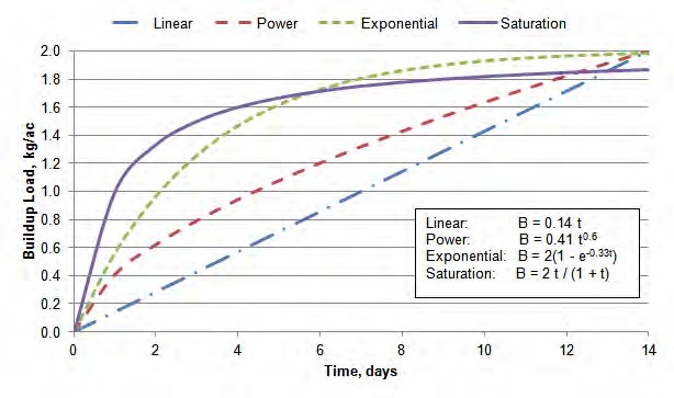
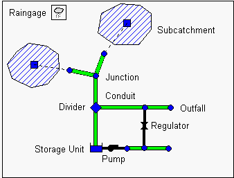
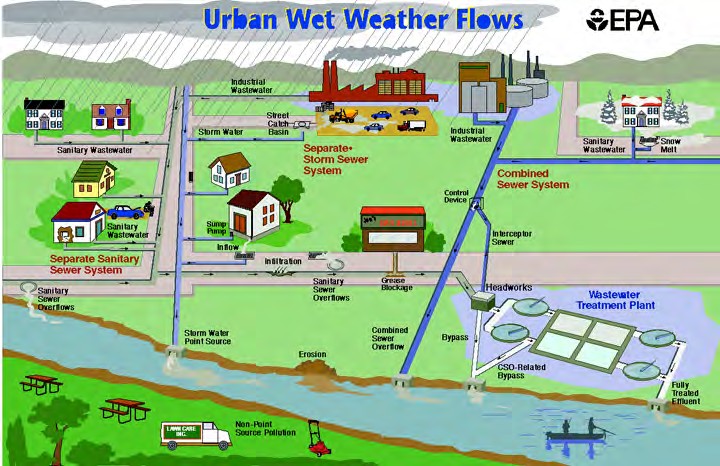
Leave a Reply