Calibration Functions for the InfoSWMM and InfoSWMM SA Calibrator
When calibrating a Stormwater management model, the goal is to determine the best set of InfoSWMM model parameters which produces the lowest overall deviation between the numerically simulated model results and the observed field data at user specified locations in the system. Observed field data can include link flow, link depth, and link velocity measurements. These measurements could be taken at one or more links in the system.
Grouping is very useful in the calibration process. InfoSWMM and InfoSWMM SA calibrator has five group types: Subcatchment group, soil group, aquifer group, RDII group, and conduit group. Grouping has to be made accounting for similarity in the characteristics of the elements. For example, if the modeler is interested in calibrating subcatchment width s/he may need to group subcatchments depending on their similarity in shape/size so that subcatchments in the group may use the same multiplying factor during the calibration. To calibrate Manning’s roughness parameter for conduits, one may need to group conduits together depending on similarity in their characteristics such as material, date of installation, location, and diameter. It is assumed that all elements within a group will have an identical multiplying factor for the parameter being calibrated. The multiplying factor would be multiplied by the original parameter value assigned to each of the individual elements to determine actual value of parameter to be used during the calibration process.
InfoSWMM Calibrator casts the calibration problem as an implicit nonlinear optimization problem, subject to explicit inequality and equality constraints. It computes optimal model parameters within user-specified bounds, such that the deviation between the model predictions and field measurements is minimized. The optimal model calibration problem is thus governed by an objective function and its associated set of constraints.
1.1 OBJECTIVE FUNCTIONS
The objective of the optimal calibration problem is to minimize the numerical discrepancy between the observed and predicted values of link flow, link depth, and/or link velocity at various locations in the system. Any of the following nine different mathematical objective functions can be used in InfoSWMM Calibrator.
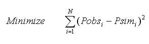
Root Mean Square Error (RMSE)

In the ideal condition when corresponding observed and simulated values exactly match, value of RMSE will be zero.
Simple Least Square Error (SLSE)
This performance evaluation function could assume values ranging from zero (best fit) to ∞ (poor fit), and it tends to favor large errors and large (i.e., peak) flows.
Mean Simple Least Square Error (MSLSE)
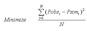
This performance evaluation function could assume values ranging from zero (best fit) to ∞ (poor fit), and it tends to favor large errors and large (i.e., peak) flows.
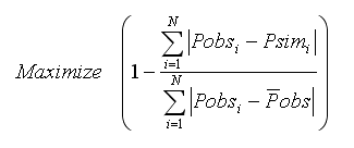
Difference in Total Volume
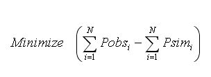
Difference in total volume could range from -∞ (poor performance) to ∞ (poor performance), the ideal value being zero (i.e., exact match between total simulated volume and total observed volume).
Nash-Sutcliffe Efficiency Criterion
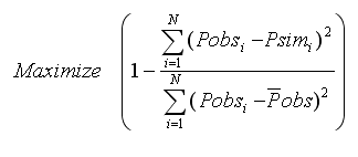
This efficiency criterion could assume values from -∞ (poor performance) to 1 (perfect model).
R-Square (R2)
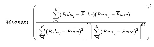
R2 value varies from zero (indicates worst fit) to unity (indicates perfect fit).
Modified Coefficient of Efficiency
The modified coefficient of efficiency could assume values from -∞ (poor performance) to 1 (perfect model).
Dimensionless Root Mean Square Error (DRMSE)
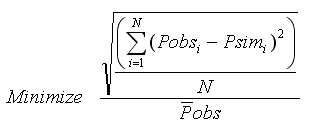
In the ideal condition when corresponding observed and simulated values exactly match, value of DRMSE will be zero.
Dimensionless Simple Least Square Error (DSLSE)
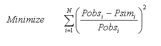
where N designates the total number of measurements available, Pobsi represents the observed measurement values at time i; Psimi is the model simulated values at time i; is mean of the measured values; is mean of the simulated values.
This performance evaluation function could assume values ranging from zero (best fit) to ∞ (poor fit), and it tends to be independent of length of records and it favor large errors and large (i.e., peak) flows.
It is believed that complete assessment of model performance should include at least one relative error measure (e.g., modified coefficient of efficiency) and at least one absolute error measure (e.g., root mean square error) with additional supporting information (e.g., a comparison between the observed and simulated mean and standard deviation).
The number of field measurements defining the objective function must be greater than or equal to the number of calibration variables. It is expected that the accuracy of the model calibration would be increased by the use of a large number of field measurements. The decision variables could be any one or more of about fifty nfoSWMM H2OMap SWMM InfoSWMM SA parameters. These decision variables are automatically adjusted to minimize the objective function selected while satisfying a set of implicit and explicit constraints.
1.2 IMPLICIT SYSTEM CONSTRAINTS
The implicit constraints on the system correspond to equations that govern/simulate the underlying hydrologic, hydraulic and water quality processes including conservation of mass and conservation of momentum at various scales such as node, and/or link, and/or the entire system. Each function call to nfoSWMM H2OMap SWMM InfoSWMM SA with a set of decision variables returns the simulated values for link flow, link depth, and link velocity that will be compared with corresponding measured data.
1.3 EXPLICIT CONSTRAINTS
The explicit bound constraints are used to set minimum (lower) and maximum (upper) limits on the calibrated nfoSWMM H2OMap SWMM InfoSWMM SA parameters. For example, for each conduit group G (where a single conduit may constitute a group) Manning’s roughness coefficient for a conduit in the group may be bound by an explicit inequality constraint as follows:

where kmin designates the lower bound multiplier (minimum value of a multiplier) for roughness coefficient of conduits in conduit group G; kmax represents the upper bound multiplier (maximum value of a multiplier) for roughness coefficient of conduits in conduit group G; and n is roughness coefficient value for conduit i in group G. Please note that each of the conduits in group G could take different values of n. The only value that is same for all conduits in the group is the multiplier k.
It should be noted that the choice of grouping may greatly affect the calculated parameter values as well as the convergence accuracy. It is also expected that the final calculated parameters, will be close to the actual values (i.e., optimal/near optimal values) although they may not be “exact” or absolute optima.