Example 1. Post-Development Runoff in InfoSWMM and InfoSWMM SA
This first example demonstrates how to construct a hydrologic model of an urban catchment and use it to compare stormwater runoff under both pre- and post-development conditions. It illustrates the process of spatially dividing a catchment into smaller computational units, called Subcatchments, and discusses the characteristics of these Subcatchments that InfoSWMM H2OMap SWMM InfoSWMM SA uses to transform rainfall into runoff. This example considers runoff only. Flow routing of runoff through the drainage pipes and channels contained within the catchment is addressed in Example 2.
Models of this type are very common in practice. Many local stormwater ordinances and agencies require that new developments limit peak runoff flows relative to those under pre-development conditions. To meet environmental sustainability objectives, similar criteria are being applied to total runoff volume as well.
1.1 Problem Statement
Figure 1-1 is a contour map of a 29 acre natural catchment area where a new residential development is planned. This undeveloped area is primarily pasture land that has a silt loam soil type. Figure 1-2 shows the proposed development for this site. With the exception of the depressions located in the parkland area, no major changes in topography are expected. This implies that future streets will, in general, follow the natural slope. However, the residential lots will be graded toward the street at a slope of 2% so they can drain easily. The developed site will drain to a stream through a culvert under the street located on the southeast side of the site, which is considered to be the outlet point of the catchment.
The objective is to estimate the stormwater discharges at the catchment’s outlet and compare them to the ones generated prior to urbanization. The approach typically employed in stormwater drainage manuals will be used, which is to compute the hydrologic response of the catchment to a series of synthetic design storms associated with different return periods. The design storms used here will be for a 2-hour event with return periods of 2, 10, and 100 years. Most of the parameter values used in this example were taken from tables published in the InfoSWMM H2OMap SWMM InfoSWMM SA Users Guide. These were supplemented with design guidelines published by the Denver Urban Drainage and Flood Control District (UDFCD) (UDFCD, 2001).
Two models will be built: one that represents the catchment in its current undeveloped condition and one that represents the catchment after it is fully developed. Because this is an initial estimation of the discharges at the outlet of the catchment under its current and future conditions, no channelized flows will be defined and only runoff as overland flow will be simulated. Example 2 in this manual will add a conveyance system of swales, channels, and culverts to this model.

Figure 1-1. Undeveloped site
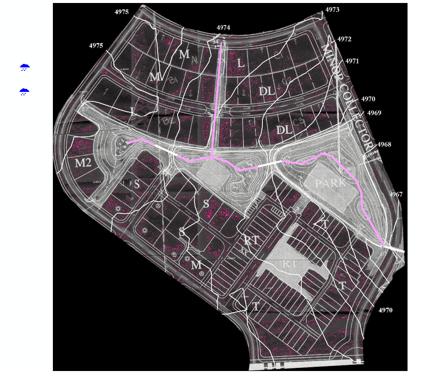
Figure 1-2. Developed site
1.2 System Representation
SWMM is a distributed model, which means that a study area can be subdivided into any number of irregular Subcatchments to best capture the effect that spatial variability in topography, drainage pathways, land cover, and soil characteristics have on runoff generation. An idealized Subcatchment is conceptualized as a rectangular surface that has a uniform slope and a width W that drains to a single outlet channel as shown in Figure 1-3. Each Subcatchment can be further divided into three subareas: an impervious area with depression (detention) storage, an impervious area without depression storage and a pervious area with depression storage. Only the latter area allows for rainfall losses due to infiltration into the soil.


Figure 1-3. Idealized representation of a Subcatchment

The hydrologic characteristics of a study area’s Subcatchments are defined by the following set of input parameters in InfoSWMM H2OMap SWMM InfoSWMM SA:
Area
This is the area bounded by the Subcatchment boundary. Its value is determined directly from maps or field surveys of the site or by using InfoSWMM H2OMap SWMM InfoSWMM SA Auto-Length tool when the Subcatchment is drawn to scale on InfoSWMM H2OMap SWMM InfoSWMM SA study area map.
Width
The width can be defined as the Subcatchment’s area divided by the length of the longest overland flow path that water can travel. If there are several such paths then one would use an average of their lengths to compute a width.
In applying this approach you must be careful not to include channelized flow as part of the flow path. In natural areas, true overland flow can only occur for distances of about 500 feet before it begins to consolidate into rivulet flow. In urbanized catchments, true overland flow can be very short before it is collected into open channels or pipes. A maximum overland flow length of 500 feet is appropriate for non-urban catchments while the typical overland flow length is the length from the back of a representative lot to the center of the street for urban catchments. If the overland flow length varies greatly within the Subcatchment, then an area-weighted average should be used.
Because it is not always easy to accurately identify all of the overland flow paths within a Subcatchment, the width parameter is often regarded as a calibration parameter whose value can be adjusted to produce a good match between observed and computed runoff hydrographs.
Slope
This is the slope of the land surface over which runoff flows and is the same for both the pervious and impervious surfaces. It is the slope of what you consider to be the overland flow path or its area-weighted average if there are several such paths in the Subcatchment.
Imperviousness
This is the percentage of the Subcatchment area that is covered by impervious surfaces, such as roofs and roadways, through which rainfall cannot infiltrate. Imperviousness tends to be the most sensitive parameter in the hydrologic characterization of a catchment and can range anywhere from 5% for undeveloped areas up to 95% for high-density commercial areas.
Roughness Coefficient
The roughness coefficient reflects the amount of resistance that overland flow encounters as it runs off of the Subcatchment surface. Since InfoSWMM uses the Manning equation to compute the overland flow rate, this coefficient is the same as Manning’s roughness coefficient n. Separate values are required for the impervious and pervious fractions of a Subcatchment since the pervious n is generally an order of magnitude higher than the impervious n (e.g., 0.8 for dense wooded areas versus 0.012 for smooth asphalt).
Depression Storage
Depression storage corresponds to a volume that must be filled prior to the occurrence of any runoff. Different values can be used for the pervious and impervious areas of a Subcatchment. It represents initial abstractions such as surface ponding, interception by flat roofs and vegetation, and surface wetting. Typical values range between 0.05 inches for impervious surfaces to 0.3 inches for forested areas.
Percent of Impervious Area Without Depression Storage
This parameter accounts for immediate runoff that occurs at the beginning of rainfall before depression storage is satisfied. It represents pavement close to the gutters that has no surface storage, pitched rooftops that drain directly to street gutters, new pavement that may not have surface ponding, etc. By default the value of this variable is 25%, but it can be changed in each Subcatchment. Unless special circumstances are known to exist, a percent imperviousness area without depression storage of 25% is recommended.
Infiltration Model
Three different methods for computing infiltration loss on the pervious areas of a Subcatchment are available in InfoSWMM. They are the Horton, Green-Ampt and Curve Number models. There is no general agreement on which model is best. The Horton model has a long history of use in dynamic simulations, the Green-Ampt model is more physically-based, and the Curve Number model is derived from (but not the same as) the well-known SCS Curve Number method used in simplified runoff models.
The Horton model will be used in the current example. The parameters for this model include (more information on the Horton method can be found in the InfoSWMM Users Guide and on-line help as well as in the literature):
- Maximum infiltration rate: This is the initial infiltration rate at the start of a storm. It is difficult to estimate since it depends on the antecedent soil moisture conditions. Typical values for dry soils range from 1 in/h for clays to 5 in/h for sands.
- Minimum infiltration rate: This is the limiting infiltration rate that the soil attains when fully saturated. It is usually set equal to the soil’s saturated hydraulic conductivity. The latter has a wide range of values depending on soil type (e.g., from 0.01 in/hr for clays up to 4.7 in/hr for sand).
- Decay coefficient: This parameter determines how quickly the infiltration rate “decays” from the initial maximum value down to the minimum value. Typical values range between 2 to 7 hr-1.
Precipitation Input
Precipitation is the principal driving variable in a rainfall-runoff-quantity simulation. The volume and rate of stormwater runoff depends directly on the precipitation magnitude and its spatial and temporal distribution over the catchment. Each Subcatchment in InfoSWMM H2OMap SWMM InfoSWMM SA is linked to a Rain Gage object that describes the format and source of the rainfall input for the Subcatchment.
1.3 Model Setup – Undeveloped Site
The InfoSWMM H2OMap SWMM InfoSWMM SAmodel for the undeveloped site is depicted in Figure 1‑4. It consists of a rain gage ‘RAINGAGE’ that provides precipitation input to a single Subcatchment ‘S0’ whose runoff drains to outfall node ‘O1’. Note that the undeveloped site contour map has been used as a backdrop image on which the Subcatchment outline has been drawn. The corresponding scenario in ‘InfoSWMM Applications.mxd’ is EX1-PRE.
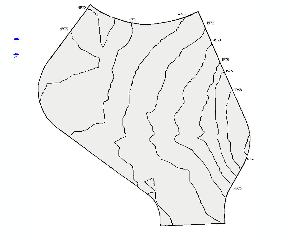
Figure 1-4. InfoSWMM representation of the undeveloped study area
Subcatchment Properties
According to the site’s contour map, its topography is fairly homogenous and no well-defined channels exist within the basin which means that mainly overland flow takes place. There are no roads or other local impervious areas and the type of soil is similar throughout the watershed (Sharpsburg silt loam). Therefore, no disaggregation is required based on the spatial distribution of catchment properties. The single Subcatchment S0 drains to the free outfall node O1 whose elevation is 4967 ft.
The area shown in Figure 1-4 is not the entire pre-development natural catchment. It has been bounded by the post-development roadways to come so that comparisons between the two conditions (developed and undeveloped) can be made.
The properties assigned to the single Subcatchment S0 are summarized in Table 1-1. Their values were developed on the basis of the undeveloped site being primarily pasture land containing a silt loam soil. Parameter values for this soil type can be found in the InfoSWMM Users Guide and the UDFCD Guidance Manual.
The Subcatchment’s area was determined using InfoSWMM’s Auto Area Calculation feature. The Subcatchment width was arrived at by first assuming a maximum overland-flow length of 500 ft, as recommended for undeveloped areas. By the time runoff has travelled this distance it has consolidated into rivulets and therefore no longer behaves as overland flow over a uniform plane. Based on this assumption, the Subcatchment was divided into subareas with flow-path lengths of 500 feet or less. Figure 1-5 shows that there were three such areas whose flow-path lengths are each 500 ft. Thus, the average flow length is also 500 ft. When the total Subcatchment area of 28.94 acres (1,260,626 ft2) is divided by the average flow length the resulting Subcatchment width is 2,521 ft. The average slope of the Subcatchment was derived from the area-weighted average of the slopes of the three sub-areas that comprise the overland flow paths as shown in Figure 1-5 and Table 1-2. Its value is 0.5.
Table 1-1. Properties of the undeveloped Subcatchment
| Property | Value | Property | Value |
| Area | 28.94 ac | Depression storage, pervious areas | 0.3 in. |
| Width | 2521 ft | Depression storage, impervious area | 0.06 in. |
| Slope | 0.5 % | % of impervious area without depression storage | 25% |
| Imperviousness | 5 % | Maximum infiltration rate | 4.5 in./hr |
| Roughness coefficient, impervious areas | 0.015 | Minimum infiltration rate | 0.2 in./hr |
| Roughness coefficient, pervious areas | 0.24 | Infiltration decay coefficient | 6.5 hr-1 |
Figure 1-5. Computation of width of the undeveloped Subcatchment
The Horton method was selected as the infiltration model for this analysis. The values assigned to its parameters are typical of those for a silt loam soil as found in this watershed and are listed in Table 1-1. It is strongly recommended to use any available site-specific data from the study area BEFORE relying on values from the literature.
Table 1-2. Flow lengths and slopes of the undeveloped Subcatchment
| Sub-Area | Flow Path Length (ft) | Associated Area (Ai) (ac) | Upstream Elevation (ft) | Downstream Elevation (ft) | Elevation Difference (ft) | Slope (Si) (%) |
| 1 | 500 | 11.13 | 4974.8 | 4973.0 | 1.8 | 0.4% |
| 2 | 500 | 14.41 | 4973.0 | 4970.0 | 3.0 | 0.6% |
| 3 | 500 | 3.40 | 4970.0 | 4967.0 | 3.0 | 0.6% |
| Average | 500 | 0.5%1 |

Rain Gage Properties
The properties of RAINGAGE describe the source and format of the precipitation data that are applied to the study area. In this example, the rainfall data consist of three synthetic design events that represent the 2-, 10- and 100-year storms of 2-hour duration. Each storm is represented by a separate time series object in the InfoSWMM model that consists of rainfall intensities recorded at a 5 minute time-interval. The time series are named 2-yr, 10-yr and 100-yr, respectively and are plotted in Figure 1-6. The total depth of each storm is 1.0, 1.7, and 3.7 inches, respectively. These design storms were selected by the City of Fort Collins, CO to be used with InfoSWMM (City of Fort Collins, 1999).

Figure 1-6. Design storm hyetographs
1.4 Model Results – Undeveloped Site
Analysis Options
Table 1-3 shows the analysis options used to run the model. Three runs of the model were made, one for each design storm event. To analyze a particular storm event one only has to change the Series Name property of the rain gage to the rainfall time series of interest. Alternatively, Figure 1-7 shows a separate scenario can be established for running each rainfall event for the undeveloped case for this example.
Each scenario has its own Raingage Set so that RAINGAGE can point to a different rainfall time series for each scenario. Each scenario also uses custom field created in the information tables with a Query Set to ensure that the proper facilities are selected for each scenario.
Table 1-3. Analysis options
| Option | Value | Explanation |
| Flow units | CFS | U.S. customary units used throughout |
| Routing Method | Kinematic wave | Must specify a routing method, but it is not used in the overland flow computations in this example |
| Start analysis time and date | 01/01/07 – 00:00 | Not important for single event simulation |
| Start reporting time and date | 01/01/07 – 00:00 | Start reporting results immediately |
| End analysis time and date | 01/01/07 – 12:00 | 12 hrs. of simulation (storm duration is 2 hrs.) |
| Reporting time step | 1 minute | Good level of detail in results for a short simulation |
| Runoff dry-weather time step | 1 hour | Not important for single event simulation |
| Runoff wet-weather time step | 1 minute | Should be less than the rainfall interval |
| Routing time step | 1 minute | Should not exceed the reporting time step |

Figure 1-7. Scenario setup for Example 1 pre-development condition
Batch Run
Instead of simulating the three scenarios separately, the Batch Simulation Manager was used to simulate all three scenarios at the same time. Figure 1-8 shows the setup of the tool to run the appropriate scenarios together.
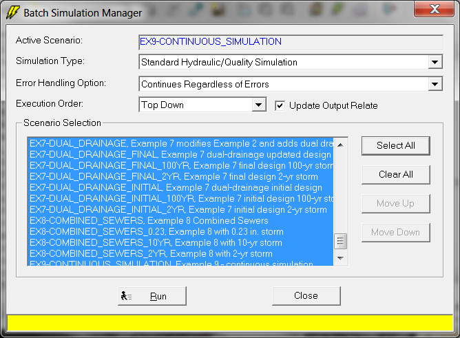
Figure 1-8. Setup of Batch Simulation Manager to run all three scenarios
Simulation Results
Since all three scenarios have been simulated, there are output results available for all three. Figure 1-9 shows outfall hydrographs for all three scenarios plotted on the same graph. This can be done by opening the outfall hydrograph for the current scenario and then click the Compare Graph button ( ![]() ) and selecting output from the other two simulated scenarios. Rainfall can be plotted on the same graph by clicking the Mix Graph button (
) and selecting output from the other two simulated scenarios. Rainfall can be plotted on the same graph by clicking the Mix Graph button ( ![]() ) and selecting the Graph Data of Another Element option and selecting Subcatchment S0.
) and selecting the Graph Data of Another Element option and selecting Subcatchment S0.
Note the significant increase in the peak discharge as the return period increases and how sensitive it is to the rainfall intensity. The rate at which the discharge volume increases is much greater than the rate at which the rainfall volume changes for different return periods. This is because the soil becomes more saturated during larger storms resulting in more of the rainfall becoming runoff.
Table 1-4 compares the peak rainfall intensity, total rainfall, total runoff volume, runoff coefficient, peak runoff discharge and total infiltrated volume for each design storm. Additionally, the last column report Manager.

Figure 1-9. Rainfall and outfall hydrograph for three scenarios
Table 1-4. Summary of results for the undeveloped site
| Design Storm | Peak Rainfall (in./hr) | Total Rainfall (in.) | Runoff Volume (in.) | Runoff Coeff. (%) | Peak Runoff (cfs) | Total Infiltration (in.) | % of Rainfall Infiltrated |
| 2-yr | 2.85 | 0.978 | 0.047 | 4.8 | 4.14 | 0.93 | 95.1 |
| 10-yr | 4.87 | 1.711 | 0.22 | 13.1 | 7.34 | 1.48 | 86.5 |
| 100-yr | 9.95 | 3.669 | 1.87 | 50.8 | 31.6 | 1.80 | 49.1 |
1.5 Model Setup – Developed Site
The increase in impervious surface and reduction of overland flow length are the main factors affecting the hydrologic response of a catchment when it becomes urbanized. The reduction in infiltrative surface creates additional surface runoff as well as higher and faster peak discharges. In this section, the runoff hydrology of our example site will be modeled in its post-development condition. The corresponding scenario in ‘InfoSWMM Applications.mxd’ is EX1-POST with three ‘child’ scenarios, one for each design storm. Again, the focus will be on just the rainfall-runoff transformation and overland flow processes. Routing through channelized elements will be covered in Example 2.
Catchment Discretization
In the urbanized catchment there are channelized elements (gutters and swales) that conduct runoff to the site’s outlet. The partitioning of the study area into individual Subcatchments depends not only on the spatial variability in land features but also on the location of the channelized elements. Inspection of the developed site plan for the example study area (see Figure 1-2) suggests that a total of seven Subcatchments would be sufficient to represent both the spatial differences in planned land uses and the location of channelized elements within the site. The Subcatchment boundaries were determined by aggregating together sub-areas whose potential overland flow paths share a common direction and drain to the same collection channel. The resulting discretization is shown in Figure 1-10.
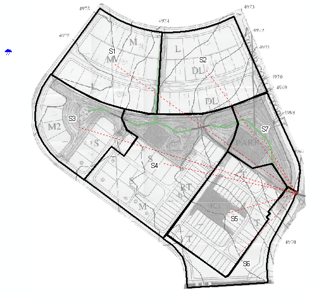
Figure 1‑10. Discretization of the developed site into Subcatchments
Figure 1‑10 shows all of the Subcatchments discharging their overland flow directly into the watershed’s outlet node, O1. In reality, the discharge outlet of each Subcatchment should be the point where its runoff enters the channelized drainage system. However, since this example does not consider routing through any channelized elements in the watershed (Example 2 covers this issue) it is acceptable to use the study area’s outlet node (O1) as a common outlet for all of the Subcatchments. The elevation of this point is 4962 ft, which corresponds to the bottom elevation of a planned culvert under the street.
Geometric Parameters
Table 1-5 lists the area, flow path length, width, slope and imperviousness of each Subcatchment. The areas were computed using InfoSWMM’s Auto-Area tool as the outline of each Subcatchment was traced on the scaled backdrop image.
Table 1-5. Geometric properties of the Subcatchments in the developed site
| Subcatchment | Area (ac) | Flow Length (ft) | Width (ft) | Slope (%) | Percent Impervious |
| S1 | 4.55 | 125 | 1587 | 2.0 | 56.8 |
| S2 | 4.74 | 125 | 1653 | 2.0 | 63.0 |
| S3 | 3.74 | 112 | 1456 | 3.1 | 39.5 |
| S4 | 6.79 | 127 | 2331 | 3.1 | 49.9 |
| S5 | 4.79 | 125 | 1670 | 2.0 | 87.7 |
| S6 | 1.98 | 125 | 690 | 2.0 | 95.0 |
| S7 | 2.33 | 112 | 907 | 3.1 | 0.0 |
Figure 1-11 illustrates how the overland flow path length was estimated for Subcatchment S2 which consists entirely of residential lots. This Subcatchment can be represented as a rectangular area with an overland flow length equal to the distance from the back of a typical lot to the middle of the street (125 ft in this case). InfoSWMM’s width parameter can then be computed as the area (4.74 ac = 206,474.4 ft2) divided by the overland flow length, which results in a value of 1650 ft.
In contrast to S2, Subcatchments S3 and S4 contain both residential lots and grass-covered areas. Their overland flow lengths are computed as an area-weighted average of the flow lengths across each type of area as shown in Figure 1‑12. Their widths are then found by dividing their areas by their overland flow lengths.
Slopes characterizing overland flow in mostly urbanized Subcatchments will be the lot slope, which is usually about 2%. By way of illustration, Figure 1‑12 shows how the slopes of Subcatchments S3 and S4 correspond to the area-weighted average of the slope of the overland flow paths over both the residential lots and the grass-covered areas.

Figure 1-11. Definition of overland flow length and slope for Subcatchment S2

Figure 1-12. Width and slope computation for Subcatchments S3 (a) and S4 (b)
Imperviousness
The imperviousness parameter in InfoSWMM is the effective or directly connected impervious area, which is typically less than the total imperviousness. The effective impervious area is the impervious area that drains directly to the stormwater conveyance system, e.g. a gutter, pipe or swale. Ideally, the imperviousness should be measured directly in the field or from orthophotographs by determining the percent of land area devoted to roofs, streets, parking lots, driveways, etc. When these observations are not available, it is necessary to use other methods. A conservative approximation that tends to overestimate runoff discharges is to use runoff coefficients as the imperviousness value. A runoff coefficient is an empirical-constant value that represents the percentage of rainfall that becomes runoff. Using the runoff coefficient to represent the percent imperviousness of a Subcatchment results in a higher estimate of impervious area because the value is calculated from the runoff of both the impervious and pervious areas of the Subcatchment. For purely illustrative purposes, runoff coefficients will be used in this example to estimate the imperviousness for each Subcatchment within the developed watershed. The steps involved are as follows:
1. Identify all of the major land uses that exist within the Subcatchment.
2. Compute the area Aj devoted to each land use j in the Subcatchment.
3. Assign a runoff coefficient Cj to each land use category j. Typical values are available in drainage criteria and basic literature (see for example UDFCD, 2001; Akan, 2003). Pervious areas are assumed to have a runoff coefficient of 0.
4. Compute the imperviousness I as the area weighted average of the runoff coefficients for all of the land uses in the Subcatchment, I = (ΣCjAj)/A, where A is the total area of the Subcatchment.
When this approach is applied to the current example the results listed in Table 1‑6 and Table 1‑7 are obtained. Table 1‑6 displays the various land-use categories that appear in the developed site along with their runoff coefficients. The latter were obtained from the City of Fort Collins Storm Drainage Design Criteria and Construction Standards (City of Fort Collins, (city of Fort Collins, 1984 and 1997). Table 1‑7 lists the amount of area devoted to each land use within the site’s Subcatchments. These areas were used to compute a weighted-average runoff coefficient that is used as a surrogate for the imperviousness of the given Subcatchment.
Table 1‑6. Land use categories in the developed site
| Id | Land Use | Runoff coefficient (C) |
| M | Medium density | 0.65 |
| L | Low density | 0.45 |
| DL | Duplex | 0.70 |
| M2 | Medium density | 0.65 |
| S | Apartment, high density | 0.70 |
| RT | Commercial | 0.95 |
| T | Commercial | 0.95 |
| P | Natural (park) | 0 |
Remaining Parameters
The remaining Subcatchment properties for the developed site (roughness coefficients, depression storages, and infiltration parameters) are kept the same as they were for the undeveloped condition. Likewise, the same analysis options were used to run the simulations. Refer to Table 1-1 and Table 1-3 for a listing of the parameter values used in the undeveloped condition.
Table 1-7. Land use coverage (ac) and imperviousness for Subcatchments in the developed site
| Sub-catchment | Total Area (ac) | Area M | Area L | Area DL | Area M2 | Area S | Area RT | Area T | Area P | Imperviousness (%) |
| S1 | 4.55 | 2.68 | 1.87 | 0 | 0 | 0 | 0 | 0 | 0 | 56.8 |
| S2 | 4.74 | 0 | 1.32 | 3.42 | 0 | 0 | 0 | 0 | 0 | 63.0 |
| S3 | 3.74 | 0 | 0 | 0 | 1.00 | 1.18 | 0 | 0 | 1.56 | 39.5 |
| S4 | 6.79 | 0.61 | 0 | 0 | 0 | 2.05 | 1.64 | 0 | 2.49 | 49.9 |
| S5 | 4.79 | 0 | 0 | 0 | 0 | 0 | 0.70 | 3.72 | 0.37 | 87.7 |
| S6 | 1.98 | 0 | 0 | 0 | 0 | 0 | 0 | 1.98 | 0 | 95 |
| S7 | 2.33 | 0 | 0 | 0 | 0 | 0 | 0 | 0 | 2.33 | 0 |
1.6 Model Results – Developed Site
Figure 1-13 shows the outlet hydrographs (the Total Inflow to node O1) obtained for each of the design storms under post-development conditions in the study site. As with the pre-development hydrographs, the peak runoff flow occurs close to when the peak rainfall does and there is a significant increase in peak discharge as the return period increases. Unlike the pre-development case, the post-development’s hydrographs show a more rapid decline once the rainfall ceases. This behavior can be attributed to the much larger amount of imperviousness under the post-development condition (57%) as compared to pre-development (5%). Table 1-8 summarizes the results obtained for each design storm in the same fashion that Table 1-4 did for the pre-development condition.
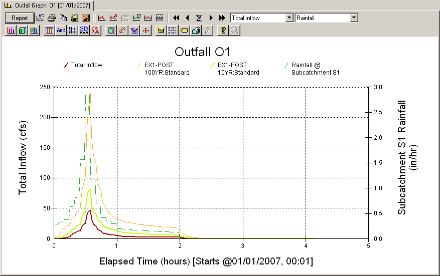
Figure 1-13. Rainfall and outfall hydrograph for three scenarios (post-development)
Table 1-8. Summary of results for post-development conditions
| Design Storm | Peak Rainfall (in./hr) | Total Rainfall (in.) | Runoff Volume (in.) | Runoff Coeff. (%) | Peak Runoff (cfs) | Total Infiltration (in.) | % of Rainfall Infiltrated |
| 2-yr | 2.85 | 0.978 | 0.53 | 54.5 | 46.7 | 0.42 | 42.9 |
| 10-yr | 4.87 | 1.711 | 1.11 | 64.7 | 82.6 | 0.58 | 33.8 |
| 100-yr | 9.95 | 3.669 | 3.04 | 82.7 | 241 | 0.61 | 16.6 |
Pre- and Post-Development Comparison
Table 1-9 compares total runoff volumes, runoff coefficients, and peak discharges computed for both the pre- and post-development conditions. For larger storm events, where infiltration plays a minor role in the runoff generation, the responses become more similar between the two cases. Total runoff volume under post-development conditions is approximately 10, 5, and 2 times greater than under pre-development conditions for the 2-yr, 10-yr, and 100-yr storms, respectively. Peak flows are about 10 times greater for both the 2-yr and 10- yr storms but only 7 times greater for the 100-yr event.
Table 1-9. Comparison of runoff for pre- and post-development conditions
| Design Storm | Total Rainfall (in.) | Runoff Volume (in.) | Runoff Coeff. (%) | Peak Runoff (cfs) | ||||||
| Pre | Post | Pre | Post | Pre | Post | |||||
| 2-yr | 0.978 | 0.047 | 0.53 | 4.8 | 54.50 | 4.14 | 46.74 | |||
| 10-yr | 1.711 | 0.22 | 1.11 | 13.1 | 64.70 | 7.34 | 82.64 | |||
| 100-yr | 3.669 | 1.87 | 3.04 | 50.8 | 82.70 | 31.6 | 240.95 | |||
1.7 Summary
This example used InfoSWMM to estimate the runoff response to different rain events for a 29 ac development that will be built in a natural area. Comparisons were made between the runoff peaks and total volume for each event for both pre- and post-developed conditions. The key points illustrated in this example were:
1. Building an InfoSWMM model for computing runoff requires that a study area be properly partitioned into a collection of smaller Subcatchment areas. These can be determined by examining the potential pathways that runoff can travel as overland flow and the location of the collection channels, both natural and constructed, that serve to intercept this runoff.
2. Initial estimates of most Subcatchment parameters can be based on published values that are tabulated for various soil types and land uses. The primary exception to this is the width parameter which should be based on the length of the overland-flow path that the runoff travels.
3. Path lengths for true overland flow should be limited to about 500 ft or to the distance at which a collection channel/pipe is reached if it is less than 500 ft.
4. Urban development can create large increases in the imperviousness, peak-runoff flow rate, and total-runoff volume.
The next case study, Example 2, will further refine the model built in this example by adding a stormwater collection system to it and routing the runoff flows through this system.