Example 6. Runoff Treatment in InfoSWMM and InfoSWMM SA

Example 6. Runoff Treatment in InfoSWMM and InfoSWMM SA

This example illustrates how to model water quality treatment in the BMPs that were used in two earlier examples to control runoff from a new residential development on a 29 acre site. Treatment of total suspended solids (TSS) is applied at both the detention pond introduced in Example 3 and the filter strips and infiltration trenches added in Example 4. The pond from Example 3 is re-designed to a smaller volume for this example to account for the runoff reduction associated with the upstream infiltration trenches. TSS removal in the detention pond is modeled as an exponential function of time and water depth. TSS removal in the filter strips and infiltration trenches is a fixed percent reduction in loading.

6.1 Problem Statement

In Example 3 a regional detention pond was designed for a 29 acre residential site to detain a water quality capture volume (WQCV) for a specific period of time and to reduce peak runoff flows to their pre-development levels. Example 4 added two different types of distributed Low Impact Development (LID) source controls throughout the site to help reduce the volume of runoff generated. Example 5 illustrated how to model total suspended solids buildup and washoff within the site without considering any TSS removal that might occur within the LIDs or the pond. These previous models will be extended to explicitly account for the removal of TSS that occurs in both the LIDs and the pond. A comparison will be made of the TSS concentrations and loads in the runoff produced by the site both with and without considering treatment.

Figure 6-1 shows the example study area with the LIDs and detention pond included. The InfoSWMM H2OMap SWMM InfoSWMM SA storage unit (SU1) that represents the detention pond as designed in Example 3 was resized (i.e. a different Storage Shape Curve is applied) for this example to incorporate a smaller Water Quality Capture Volume (WQCV) due to the runoff reduction produced by the LIDs. It was concluded from Example 4 that of the two types of LIDs modeled, infiltration trenches have the greatest impact on reducing the volume of water that needs to be treated in the pond’s WQCV. The total volume of water that can be captured by the infiltration trenches was determined to be 6,638 ft3. Because the WQCV is a requirement for the watershed as a whole, the volume captured in the infiltration trenches can be subtracted from the volume required in the regional pond, reducing it from the 24,162 ft3 required in Example 3 to 17,524 ft3 (24,162 - 6,638).

Figure 6-1. Developed site with LIDs and detention pond

The storage unit’s shape and outlet structures were redesigned to control this new WQCV and meet the general design criteria introduced in Example 3 (e.g. 40 hr drawdown time for the WQCV and peak shaving of the 2-, 10- and 100-yr storms). Table 6-1 compares the storage curve of the pond designed in Example 3 without LIDs and the pond designed for this example with LIDs. Table 6-2 does the same for the dimensions and inverts of the orifices and weirs that comprise the pond’s outlet structure. Figure 6-2 shows the general placement of the various outlets.

Table 6-1. Storage curve for the re-designed pond

This Example
Depth (ft)	0	2.2	2.3	6
Area (ft2)	10368	14512	32000	50000
Example 3
Depth (ft)	0	2.22	2.3	6
Area (ft2)	14706	19659	39317	52644

Table 6-2. Properties of the pond's re-designed outlet structure

ID	Type of Element	Event Controlled	Shape	Height h (ft)	Width b (ft)	Invert Offset z (ft)	Discharge Coefficient	Orifice or Weir Area (ft2)
Example 3
Or1	Orifice	WQCV	Side Rectangular	0.3	0.25	0	0.65	0.08
Or2	Orifice	2-yr	Side Rectangular	0.5	2.00	1.50	0.65	1.00
Or3	Orifice	10-yr	Side Rectangular	0.25	0.35	2.22	0.65	0.09
W1	Weir	100-yr	Rectangular	2.83	1.75	3.17	3.30	4.95
This Example
Or1	Orifice	WQCV	Side Rectangular	0.16	0.25	0	0.65	0.04
Or2	Orifice	2- and 10- yr	Side Rectangular	0.50	2.25	1.50	0.65	1.13
W1	Weir	100-yr	Rectangular	2.72	1.60	3.28	3.30	4.35

Figure 6-2. Schematic of the re-designed pond outlet structure

6.2 System Representation

Water Quality Treatment in LIDs

As defined in Example 4, the filter strip and infiltration trench LIDs are modeled as Subcatchments in order to represent the combined effects of infiltration and storage on storm runoff. This example will also consider their ability to reduce pollutant loads in the surface runoff they handle. There are no widely accepted mechanistic models of pollutant removal through these types of LIDs. The best one can do is to apply average removal efficiencies for specific contaminants based on field observations reported in the literature.

InfoSWMM H2OMap SWMM InfoSWMM SA can apply a constant BMP Removal Efficiency for any pollutant in the washoff generated from a particular land use. At each time step the pollutant load generated by a given land use is reduced by this user-supplied value. This reduction also applies to any upstream runoff that runs onto the Subcatchment. The LIDs added in Example 4 receive runoff from upstream Subcatchments and do not generate any pollutant load themselves. Thus it will be convenient to define a new land use, named “LID”, that is used exclusively for the LID Subcatchments and has a specific BMP Removal Efficiency for TSS associated with it.

Water Quality Treatment in Detention Ponds

Detention ponds are modeled as storage unit nodes within InfoSWMM H2OMap SWMM InfoSWMM SA. By adding Treatment Functions to the storage node’s properties, InfoSWMM H2OMap SWMM InfoSWMM SA can reduce the pollutant concentrations in the pond’s outflow. This example uses an empirical exponential decay function to model solids removal through gravity settling within a pond. For controlling the WQCV event, the pond fills relatively quickly over a period of 2 hours and then drains slowly over an extended period of 40 hours during which solids removal occurs. At some interval Δt during this drain time, and assuming homogenous concentration, the fraction of particles with a settling velocity ui that are removed would be uiΔt/d where d is the water depth. Summing over all particle settling velocities leads to the following expression for the change in TSS concentration ΔC during a time step Δt:

(6-1)

where is the total concentration of TSS particles at time t and fi is the fraction of particles with settling velocity ui. Because Σ fiui is generally not known, it can be replaced with a fitting parameter k and in the limit Equation (6-1) becomes:

(6-2)

Note that k has units of velocity (length/time) and can be thought of as a representative settling velocity for the particles that make up the total suspended solids in solution.

Integrating Equation (6-2) between times t and t+Δt, and assuming there is some residual amount of suspended solids C* that is non-settleable leads to the following treatment function for TSS in the pond:

(6-3)

Equation (6-3) is applied at each time step of the simulation to update the pond’s TSS concentration based on the current concentration and water depth.

6.3 Model Setup

The starting point for adding treatment to the runoff controls placed on the study site is the EX6-NO_TREATMENT scenario. This scenario contains the local LIDs defined in Example 4 and the redesigned storage unit and outlet structures described in section 6.1. The land uses in this file were re-calculated and re-assigned to each Subcatchment based on the discretization employed in Example 4. The washoff function for TSS is the EMC washoff function used in Example 5. The curb lengths and land uses assigned to each Subcatchment are listed in Table 6‑3. The Subcatchments treated by infiltration trenches or filter strips are marked in grey in this table.

Table 6-3. Curb lengths and land uses for LID Subcatchments

Subcatchment	Area (ac)	Curb Length (ft)	Residential_1 (%)	Residential_2 (%)	Commercial (%)
S1.1	1.21	450	100	0	0
S1.2	1.46	600	100	0	0
S1.3	1.88	630	100	0	0
S2.1	1.30	450	100	0	0
S2.2	1.50	600	0	100	0
S2.3	1.88	630	0	100	0
S3.1	1.29	0	0	0	0
S3.2	1.02	430	100	0	0
S3.3	1.38	500	0	85	0
S4.1	1.65	0	0	0	0
S4.2	0.79	400	0	100	0
S4.3	1.91	1150	36	64	0
S4.4	2.40	700	0	0	71
S5	4.79	2480	0	0	98
S6	1.98	1100	0	0	100
S7	2.33	565	0	0	0

LID Treatment

It is assumed that each filter strip and infiltration trench can provide 70% TSS removal for the runoff that passes over it. This is a typical removal observed for infiltration-based LIDs (Sansalone and Hird, 2003). A new land use, named “LID” is created with no TSS buildup function, an EMC TSS washoff function with 0 mg/L of TSS, and a TSS “BMP efficiency” of 70%. The land use assignment for each of the LID Subcatchments (S_FS_1 through S_FS_4 and S_IT_1 through S_IT_4) is set to 100% LID. As a result, all of the runoff generated from upstream Subcatchments that flow over these LID Subcatchments will receive 70% TSS removal.

Detention Pond Treatment

The removal of TSS in the detention pond is simulated using the exponential model given by Equation 6-3. One can roughly estimate what the removal constant k in this expression must be so that a targeted level of pollutant removal is achieved within a 40 hour detention time for the 0.23 in. WQCV design storm. If Equation 6-3 were applied over a 40 hour period to achieve a target TSS reduction of 95%, then an estimate of k would be:

(6-4)

where is some representative value of the pond depth during the 40 hour release period. As can be verified later on, the average depth in the pond for the 0.23 in design storm over a 40 hour duration is 0.15 ft. Using this value in the expression for k yields an estimate of 0.01 ft/hr. This value is of the same order as the 0.03 ft/hr figure quoted in US EPA (1986) that represents the 20-th percentile of settling velocity distributions measured from 50 different runoff samples from seven urban sites in EPA’s Nationwide Urban Runoff Program (NURP).

With this value of k and assuming a minimum residual TSS concentration C* of 20 mg/L, the following expression is entered into InfoSWMM’s Treatment Editor for the storage unit SU1: C = 20 + (TSS – 20) * EXP(-0.01 / 3600 / DEPTH * DT)

Note the meaning of the individual terms in this expression with respect to those in Equation (6-3): 20 is the value assumed for C*, TSS is the identifier given to the TSS concentration C for this model, 0.01/3600 is the value of k expressed in units of ft/s, DEPTH is the reserved word that InfoSWMM uses for the water depth d in feet, and DT is the reserved word that InfoSWMM uses for the routing time step Δt in seconds. When InfoSWMM sees reserved words like DEPTH and DT within a treatment expression it knows to automatically insert their current values into the expression at each time step.

The following analysis options should be used for all of the simulations made with this treatment-augmented input file:

Flow Routing Method: Dynamic Wave

Wet Weather Time Step: 1 minute

Flow Routing Time Step: 15 sec

Reporting Time Step: 1 minute

Total Duration: 2 days (48 hr)

The 48 hour duration was chosen so that the full effect of the drawdown of the WQCV in the detention pond could be observed. The resulting scenario is named EX6-TREATMENT.

6.4 Model Results

Results for several sets of comparison runs will be discussed. First, the effect of TSS treatment at the LIDs is considered. Figure 6-3 compares the TSS concentration in the treated runoff from filter strip S_FS_1 to that of the upstream runoff from Subcatchment S3.2 for the 0.1 in. storm. Also shown for reference are the runoff flows from each area. The reduction from 170 mg/L to 51 mg/L through the filter strip matches the 70 % TSS removal efficiency specified for the LID. Similar results are obtained for the remaining filter strips under all design storms.

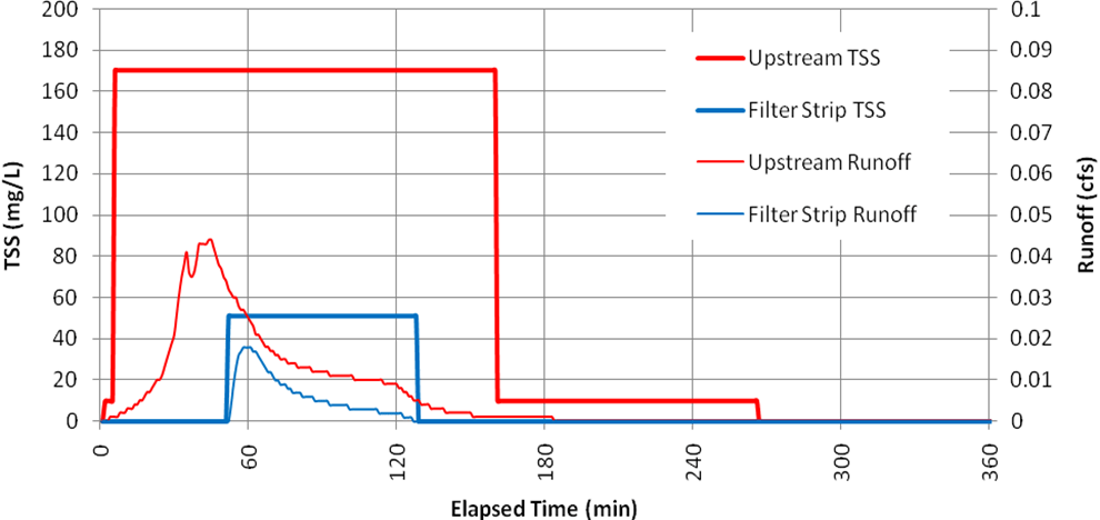
Figure 6-3. TSS and runoff reduction through filter strip S_FS_1 for the 0.1 in. storm

Figure 6-4 presents a similar comparison for the infiltration trench S_IT_4 that treats runoff from Subcatchment S2.3. These results are for the 2-yr (1 in.) event since for the smaller storms all rainfall infiltrates through the trenches. Once again note how the 70% removal causes a drop in TSS concentration from 210 mg/L down to 63 mg/L. As was the case with the filter strips, the remaining infiltration trenches show a similar behavior to that of S_IT_4.

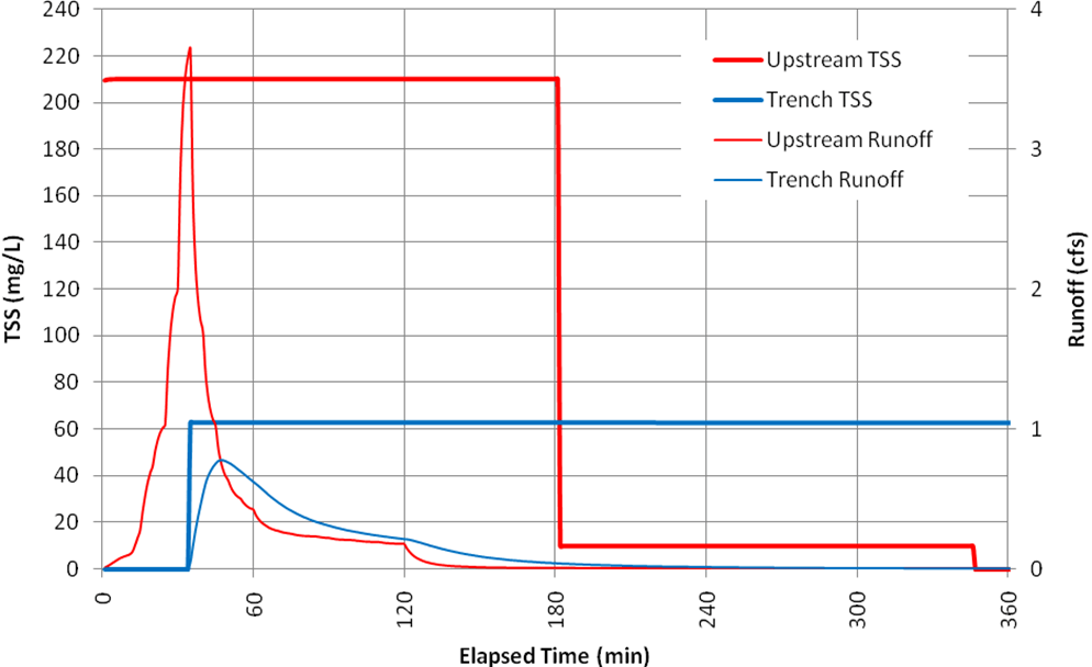
Figure 6-4. TSS and runoff reduction through infiltration trench S_IT_4 for the 2-yr storm

The next comparison is between the levels of treatment provided by the detention pond for the various design storms. Comparing the time series of pond influent TSS concentrations with the treated effluent concentrations is not particularly useful since the flow rates of these two streams are so different. Instead the pond effluent concentration, both with and without treatment will be compared for each design storm. The result is shown in Figure 6-5. These plots were made by executing a batch simulation of the model for each design storm (0.1 in., 0.23 in., and 2-year) both with the treatment function for the storage unit node SU1 and without it (i.e. all six child scenarios for Example 6). After each run a time series table of the TSS concentration at node SU1 was generated and exported to a spreadsheet program from which Figure 6-5 was generated.

The following observations can be drawn from Figure 6-5:

· With the k-value of 0.01 ft/hr, the pond behaves as designed for the WQCV storm

· (0.23 in) by removing essentially all of the settleable solids over a period of 40 hours.

· The larger the 2-hour design storm, the less effective is treatment in reducing TSS levels over time because of the deeper water depths experienced in the pond.

· For all size storms, it takes a considerable amount of time for any significant removal of TSS to occur; a 50% reduction in settleable TSS requires 10, 19, and 35 hours for the 0.1 in, 0.23 in, and 2-year storms, respectively.

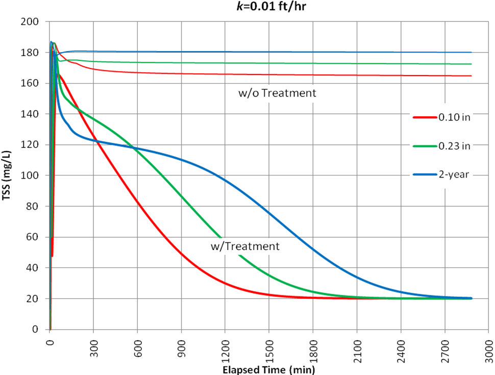
Figure 6-5. TSS concentrations in pond SU2 with and without treatment (k = 0.01 ft/hr)

Another way to evaluate treatment in the pond is to compare the TSS mass loading that it releases both with and without treatment. This is done in Figure 6-6 for the 0.23 WQCV storm. Plots for the other design storms look similar to this one. The effect of treatment on reducing the mass of TSS Release is not as significant as it was for concentration. In fact, the Continuity Quality Routing report for the run with treatment shows that of 72.6 lbs of TSS washed off for this storm event, only 15.8 lbs were removed in the pond. This yields an overall mass removal of only 21.7 %. The percent mass removals for the other design storms were 44.4 % for the 0.1 in. storm and 6 % for the 2-year (1 in.) storm. These low to moderate mass removals are a consequence of the extended time required for solids to settle in the pond during which it still is releasing an outflow.

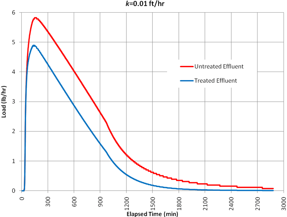
Figure 6-6. TSS mass load Release by pond SU1 for the 0.23 in storm (k = 0.01 ft/hr)

These rather modest levels of detention pond performance were computed using a removal constant k that represents particles with a very low settling velocity, below that of the lowest 20% determined from a nationwide survey. Suppose the size distribution of particles comprising the TSS washoff were larger, as reflected in a k-value of 0.3 ft/hr. This represents the 40-th percentile of the settling velocities found from the NURP study (US EPA, 1986). Figure 6-7 shows the resulting TSS concentrations in the pond discharge with this higher k-value. Figure 6-8 does the same for the TSS discharge loading for the 0.23 in. event. Table 6-4 summarizes the pond’s treatment performance for the two different k-values. These results show that uncertainty in the removal constant will significantly impact predictions of TSS removal within the detention pond. Unfortunately, as noted in US EPA (1986), there can be high variability in solids settling velocity distributions from site to site and from storm to storm within a given site. This variability makes it very difficult to make reliable estimates of detention pond treatment effectiveness.

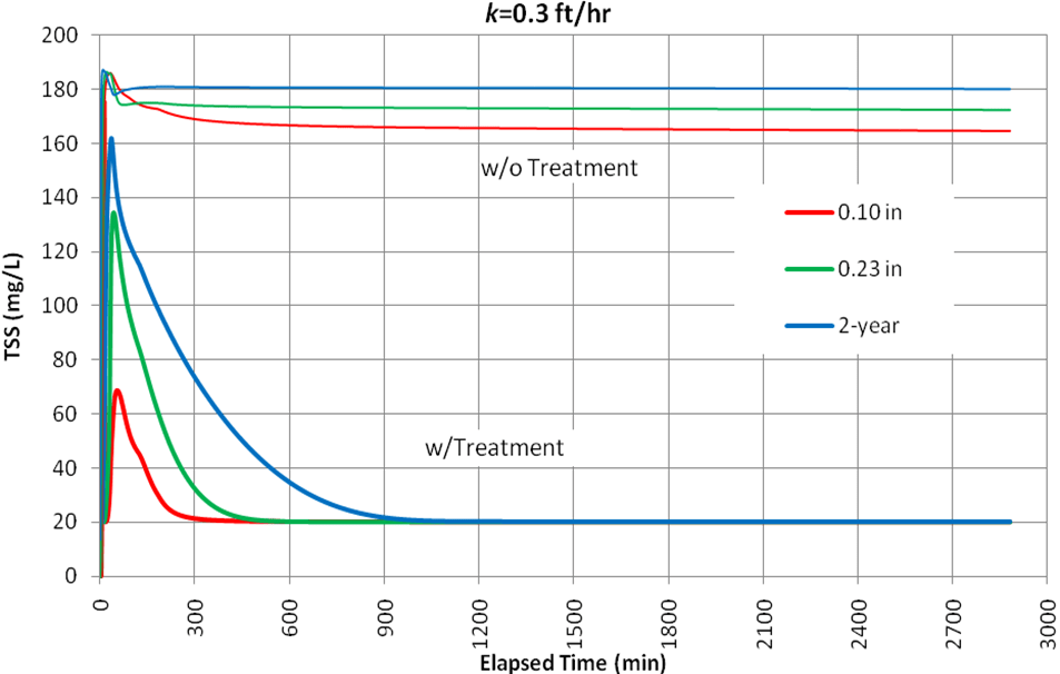
Figure 6-7. TSS concentrations in pond SU1 with and without treatment (k = 0.3 ft/hr)

Figure 6-8. TSS mass load Release by pond SU1 for the 0.23 in. storm (k = 0.3 ft/hr)

Table 6-4. Detention pond TSS treatment performance summary

	0.1 in. Storm		0.23 in. Storm		1.0 in. Storm
	k = 0.01	k = 0.3	k = 0.01	k = 0.3	k = 0.01	k = 0.3
Time to achieve 50% reduction, hr	10.0	1.0	19.0	3.0	35.0	6.0
Time to achieve full reduction, hr	30.0	7.0	40.0	10.0	>48	20.0
Overall mass removal, %	4.4	81.8	21.7	75.0	6.0	35.7

Finally, Figure 6-9 compares the total pounds of TSS discharged from the study area site for each design storm with no treatment, with just LIDs, and with both LIDs and the detention pond. These loadings can be read from the text report or from the Continuity Quality Routing report generated by running an analysis of each storm with (a) both types of treatment, (b) with the treatment function for the pond removed (LID treatment only), and (c) with the input file developed for EMC washoff in Example 5 (no treatment). The k value used in this comparison is the 0.01 ft/hr value. Note the consistent pattern of load reduction as more treatment is applied. Also note that the pond provides a lower increment of overall load reduction than do the LIDs even though the pond is a regional BMP that treats all of the catchment’s runoff while the LIDs are local BMPs that receive runoff from only 41 % of the catchment’s area. This is a result of the conservative k value used in the pond’s treatment expression. Using a higher value, which would reflect a larger particle size distribution in the runoff, would result in lower loadings from the pond.

Figure 6-9. Total TSS load discharged at site outlet under different treatment scenarios

6.5 Summary

This example showed how water quality treatment could be modeled within InfoSWMM H2OMap SWMM InfoSWMM SA. Total Suspended Solids (TSS) removal was considered in both local LID source controls as well as in a regional detention basin. The key points illustrated in this example were:

1. LID controls can be modeled as distinct Subcatchments with a single landuse that has a constant removal efficiency assigned to it. InfoSWMM H2OMap SWMM InfoSWMM SAapplies this removal efficiency to the runoff that the control receives from upstream Subcatchments.

2. Treatment within a detention pond is modeled with a user-supplied Treatment Function that expresses either the fractional removal or outlet concentration of a pollutant as a function of inlet concentration and such operational variables as flow rate, depth, and surface area.

3. An exponential treatment function was used to predict TSS removal within this example’s detention pond as a function of a removal constant and the pond’s water depth, where the removal constant reflects the settling velocity of the particles to be removed.

4. InfoSWMM H2OMap SWMM InfoSWMM SA’s use of constant removal efficiencies for LID controls makes its LID treatment performance insensitive to size of storm.

5. Treatment performance for detention ponds decreases with increasing size of storm due to an increase in pond depth. It also decreases with decreasing size distribution of the sediments that constitute the TSS in the runoff.

6. For the treatment function used in this example, the pond provided less incremental TSS load reduction than did the LIDs. This result, however, is completely dependent on the value of the removal constant used within the pond’s treatment function.

7. The large variability reported for particle settling velocities in urban runoff makes it extremely difficult to estimate a removal constant for a detention pond’s treatment function that can consistently provide reliable estimates of the pond’s treatment performance.