Example 2. Surface Drainage Hydraulics in InfoSWMM and InfoSWMM SA

Example 2. Surface Drainage Hydraulics in InfoSWMM and InfoSWMM SA

Example 1 showed how to construct a hydrologic model of an urban catchment that compared stormwater runoff under both pre- and post-development conditions. Hydraulic routing was not considered. This example will demonstrate how InfoSWMM’s hydraulic elements and flow routing methods are used to model a surface drainage system. A conveyance network will be added to the post-development model built in Example 1 and be sized to pass the 2 hour synthetic storm events with return periods of 2-, 10-, and 100-years. For simplicity, open channels (e.g. swales or gutters) will be used to convey flow. The simple routing network developed in this example will be built upon further in Example 7 where additional open channels and below-ground pipes will be added that are designed according to typical drainage design criteria.

2.1 Problem Statement

Figure 2-1 and Figure 2-2 show the InfoSWMM model layouts of the pre- and post-development study area developed in Example 1. In Figure 2‑1 the pre-development site was represented by a single Subcatchment whose width parameter was determined by assuming a maximum overland flow length of 500 ft, as recommended for undeveloped areas. For the developed case (Figure 2-2), the post-development site was discretized into seven Subcatchments, the Subcatchment widths were computed using an area-weighted average of the flow lengths across each type of area, and all Subcatchments discharged their overland flow directly to the site’s outlet, node O1 (see Section 1.5 of Example 1).

The objective of this example is to add a simple surface drainage system to the post-development site. A system of gutters, grass swales, and culverts will be designed and sized to convey the 100-yr storm. Runoff from three design storms (the 2-, 10- and 100-yr storms) will be routed through this system using the three alternative hydraulic routing methods available in InfoSWMM. The resulting outflow hydrographs at the site’s outlet will be compared to those generated in Example 1 where no hydraulic routing was used.

2.2 System Representation

InfoSWMM models a conveyance network as a series of nodes connected by links (Figure 2-3). Links control the rate of flow from one node to the next and are typically conduits (e.g. open channels or pipes) but can also be orifices, weirs or pumps. Nodes define the elevation of the drainage system and the time-varying hydraulic head applied at the end of each link it connects. The flow conveyed through the links and nodes of the model is ultimately discharged to a final node called the outfall. Outfalls can be subjected to alternative hydraulic boundary conditions (e.g. free discharge, fixed water surface, time varying water surface, etc.) when modeled with Dynamic Wave. The properties of these drainage system elements are explained in more detail in the Section 2.3.

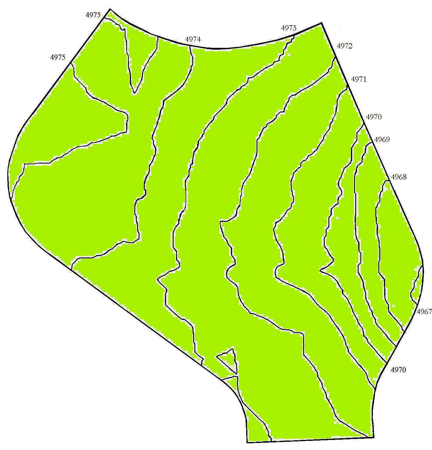
Figure 2-1. Pre-development site

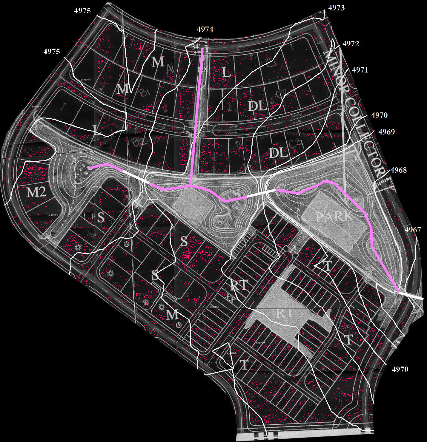
Figure 2-2. Post-development site without conveyance system

Figure 2-3. Links and Nodes

Hydraulic routing is the process of combining all inflows that enter the upstream end of each conduit in a conveyance network and transporting these flows to the downstream end over each instance of time. The resulting flows are affected by such factors as conduit storage, backwater, and pipe surcharging. InfoSWMM can perform hydraulic routing by three different methods: Steady Flow, Kinematic Wave and Dynamic Wave. These three methods are summarized below.

· Steady Flow

Steady Flow routing is an instantaneous translation of a hydrograph from the upstream end of a conduit to the downstream end with no time delay or change in shape due to conduit storage. Steady Flow routing will simply sum the surface runoff from all Subcatchments upstream of the selected node through time.

· Kinematic Wave

Kinematic Wave uses the normal flow assumption for routing flows through the conveyance system. In Kinematic Wave routing, the slope of the hydraulic grade line is the same as the channel slope. Kinematic Wave routing is most applicable to the upstream, dendritic portions of drainage systems where there are no flow restrictions that might cause significant backwater or surcharging. It can be used to approximate flows in non-dendritic systems (i.e., those that have more than one outflow conduit connected to a node) only if “flow divider” nodes are used.

· Dynamic Wave

Dynamic Wave routing is the most powerful of the flow routing methods because it solves the complete one-dimensional Saint Venant equations of flow for the entire conveyance network. This method can simulate all gradually-varied flow conditions observed in urban drainage systems such as backwater, surcharged flow and flooding. Dynamic Wave can simulate looped conduit systems and junctions with more than one link connected downstream (bifurcated systems). The ability to simulate bifurcated systems allows one to model pipes and gutters in parallel; this more advanced level of modeling will be described in Example 7.

2.3 Hydraulic Elements in InfoSWMM

All hydraulic elements modeled in InfoSWMM are classified as either nodes or links. The hierarchy of these elements is shown in Figure 2‑4 along with both the required and optional properties that characterize each element’s hydraulic behavior.

2.4 Model Setup

System Layout

Figure 2-5 shows the layout of the runoff conveyance system that will be added to the developed site. It consists of 7 grass swales, 3 culverts, and one street gutter. The objective in this example is to estimate the discharges at the outlet of the site and not design all of the elements within the entire drainage system. For this reason, only the main surface conduits that route runoff to the outlet in the aggregated model will be considered. These will purposely be oversized to ensure that all the generated runoff is conveyed to the outlet and that no flooding occurs within the site (see Example 7 for an analysis of surcharged pipes and flooded junctions). The starting point for building this model is the scenario ‘EX1-POST’ that was created in Example 1.

In Example 1, the Subcatchment widths were set to properly represent the overland flow process. All the Subcatchments were directly connected to the outlet of the study area; flows through channels were not modeled. In this example, the Subcatchment properties will remain the same as defined previously, but conduits representing the channelized flow throughout the site will be added into the model.

The definition of the conveyance system begins by specifying the location of its nodes (or junctions). A node is required wherever runoff enters the conveyance system, whenever two or more channels connect and where the channel slope or cross section changes significantly. They are also required at locations with weirs, orifices, pumps, storage, etc. (see Example 3 where orifices and weirs are used as outlets to a storage unit). The locations of the nodes for this example are shown in Figure 2‑6. They are labeled J1 through J11. The invert elevation of each node (i.e., the elevation at the bottom of the lowest connecting channel) is shown in Table 2‑1.

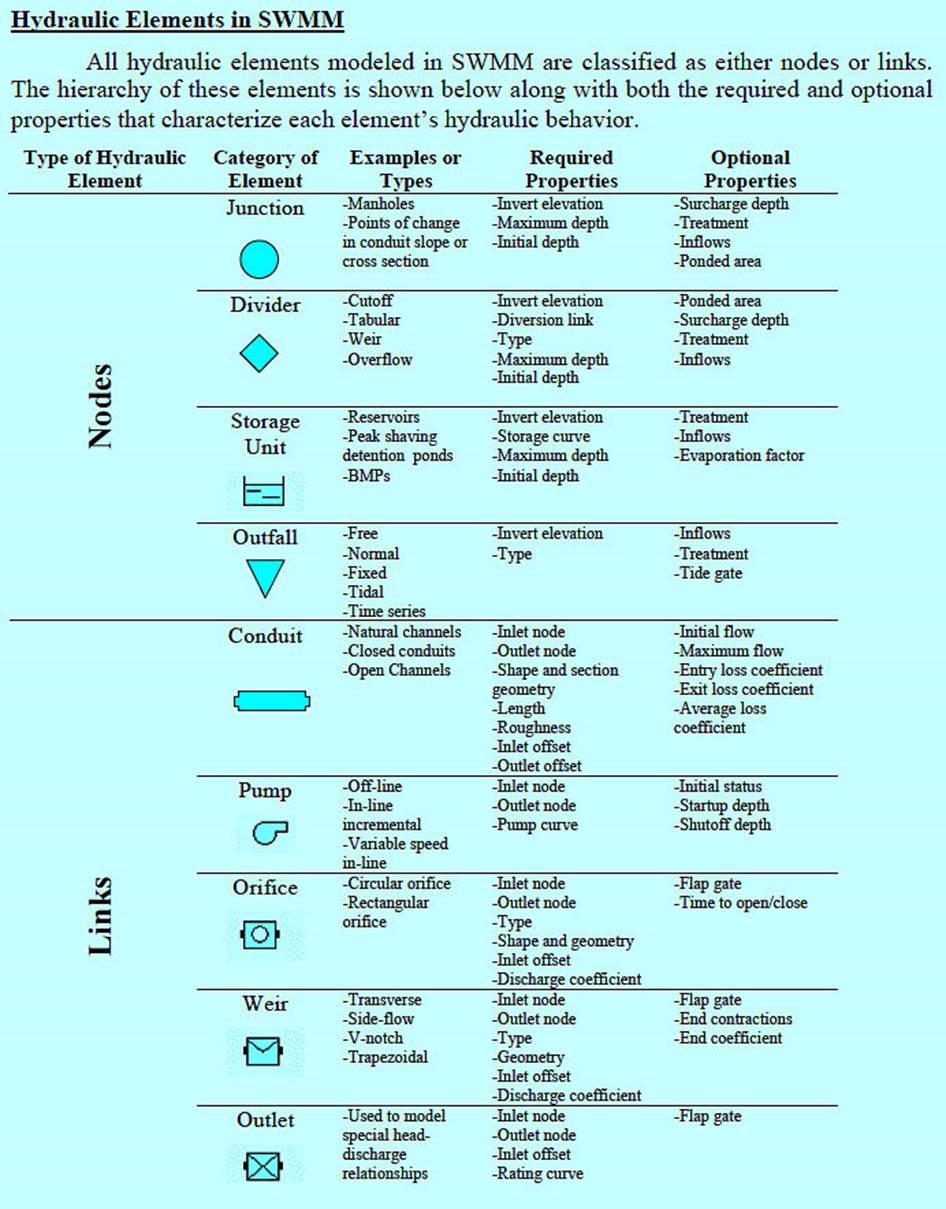
Figure 2-4. Characteristics of hydraulic elements in InfoSWMM

Figure 2-5. Post-development site with runoff conveyance added

The definition of the conveyance system continues by adding the feeder channels C1, C2 and C6 that convey runoff into the main drainage way that runs through the undeveloped park area of the site. Conduit C1 is a grass swale that drains Subcatchment S1’s runoff to the watershed’s main drainage way; Conduit C2 is a gutter that carries Subcatchment S2’s runoff to the upstream end of the culvert (C11) that discharges to the site’s outlet (O1); conduit C6 carries runoff from Subcatchment S4 into culvert C7. At this point, the elevations of the bottom bed of these channels correspond to the invert elevations of their respective upstream and downstream junctions. Their lengths are automatically determined by drawing them with Auto-Length turned on. InfoSWMM H2OMap SWMM InfoSWMM SA uses this information to compute the slope of each channel.

Figure 2-6. InfoSWMM H2OMap SWMM InfoSWMM SA representation of the post-development conveyance system

Table 2-1. Invert elevations of junctions

Junction ID	Invert Elevation (ft)
J1	4973.0
J2	4969.0
J3	4973.0
J4	4971.0
J5	4969.8
J6	4969.0
J7	4971.5
J8	4966.5
J9	4964.8
J10	4963.8
J11	4963.0

Finally, the remaining conduits C3 through C11 that comprise the main drainage way through the park to the outlet need to be defined. As before, they connect to their end nodes with no vertical offset and the Auto-Length tool is used to compute their lengths. Subcatchments S3 through S7 drain to different locations of the main drainage channel. S3 drains to the culvert (C3) at the beginning of the main drainage channel, S4 drains to the swale C6 that connects to the second culvert (C7) on the main drainage channel, S7 and S5 drain to the main drainage channel at J10, and S6 drains directly to the last culvert (C11) on the main drainage channel. Table 2-2 summarizes the outlet junction and conduit associated with each Subcatchment.

Table 2-2. Subcatchment outlets

Subcatchment	Outlet Junction	Outlet Conduit
S1	J1	C1 (Swale)
S2	J2	C2 (Gutter)
S3	J3	C3 (Culvert)
S4	J7	C6 (Swale)
S5	J10	C10 (Swale)
S6	J11	C11 (Culvert)
S7	J10	C10 (Swale)

Note that the conveyance system modeled in this example (Figure 2-6) ignores the storage and transport provided by the street gutters within each Subcatchment. In some applications, however, these conveyance elements can play a significant role and should be represented, perhaps by adding a channel within each Subcatchment that represents the aggregated effects of routing through all of its street segments. To keep the example simple, this level of detail is not included and only the major drainage channels within the site are considered.

System Properties

Properties can now be assigned to the conduits and junctions that have been defined. Table 2-3 shows the cross-sectional shapes of the three conduit types used in this example. The swale side slopes (Z1 and Z2 (horizontal:vertical)), roughness coefficient (n), bottom width (b) and height (h) of the swale section are as recommended by the UDFCD Manual (2001). The gutter cross-slopes (Z1 and Z2), roughness coefficient (n), bottom width (b) and height (h) are based on typical design practice. The culvert diameters will be sized as described in the next section to convey runoff from the 100year storm.

Table 2-4 shows the InfoSWMM properties assigned to each conduit. Conduit lengths were computed using the Auto-Length option. The inlet and outlet offset of all the conduits, with one exception, were set to zero which means that the bottom elevation of each conduit coincides with the elevation of its inlet and outlet junctions. The exception is conduit C2 (the gutter), whose outlet offset of 4 ft represents the difference in elevation between the bottom of the gutter and the channel bed in the park. The diameters of the three circular culverts will be determined in the next section.

Table 2-4. Conduit properties

Conduit ID	Type of Conduit	Inlet Node	Outlet Node	Length (ft)	h (ft) or D (ft)	b (ft)	Z1	Z2
C1	Swale	J1	J5	185	3	5	5	5
C2	Gutter	J2	J11	526	1	0	.0001	25
C3	Culvert	J3	J4	109	TBD	-	-	-
C4	Swale	J4	J5	133	3	5	5	5
C5	Swale	J5	J6	207	3	5	5	5
C6	Swale	J7	J6	140	3	5	5	5
C7	Culvert	J6	J8	95	TBD	-	-	-
C8	Swale	J8	J9	166	3	5	5	5
C9	Swale	J9	J10	320	3	5	5	5
C10	Swale	J10	J11	145	3	5	5	5
C11	Culvert	J11	O1	89	TBD	-	-	-

TBD = To Be Determined

Because the conduits are all surface channels and not buried pipes, it is sufficient to set the maximum depth of all the junctions as zero. This will cause InfoSWMM to automatically set the depth of each junction as the distance from the junction’s invert to the top of the highest conduit connected to it. Thus, junction flooding (the only flooding allowed by InfoSWMM) will occur when the channel capacity is exceeded. Finally, the outfall node O1 is defined as a free outfall with an elevation of 4962 ft. The resulting scenario in ‘InfoSWMM Applications.mxd’ is EX2-POST.

2.5 Model Results

Culvert Sizing

Before InfoSWMM’s alternative routing methods are compared, the diameters of the three culverts in the conveyance system must be determined. This is done by finding the smallest available size for each culvert from those listed in Table 2-5 that will convey the runoff from the 100-year, 2-hr design storm without any flooding. This process involves the following steps:

1. Start with each culvert at the largest available diameter.

2. Make a series of InfoSWMM runs, reducing the size of conduit C3 until flooding occurs. Set the size of C3 to the next larger diameter.

3. Repeat this process for conduit C7 and then for C11.

Note that one proceeds systematically from upstream to downstream, making sure that each culvert in turn is just big enough to handle the flow generated upstream of it. This procedure is appropriate because there is no flooding under the baseline condition (with the culverts at their maximum possible size). The approach should not necessarily be applied when pipe diameters have to be enlarged (or when there is flooding under the baseline condition). It is very common to find design situations in which changes downstream have significant effects upstream, so that a minor change in the diameter of a pipe located downstream may solve flooding problems upstream.

Table 2-5. Available culvert sizes

Diameter (ft)	Diameter (in)	Diameter (ft)	Diameter (in)	Diameter (ft)	Diameter (in)	Diameter (ft)	Diameter (in)
1.00	12	2.00	24	3.00	36	4.00	48
1.25	15	2.25	27	3.25	39	4.25	51
1.50	18	2.50	30	3.50	42	4.50	54
1.75	21	2.75	33	3.75	45	4.75	57

These culvert-sizing runs are made using the EX2-POST_100YR scenario with the routing method set to KW (Kinematic Wave), the Rain Gage’s time series set to 100-yr, and the following set of time steps: 1 minute for reporting, 1 h for dry weather, 1 minute for wet weather and 15 s for routing. Note that the routing time step is somewhat stringent for the drainage system being modeled and the routing method used (KW). It is used here, however, because Dynamic Wave routing will be used later in this example and it typically requires smaller time steps than Kinematic Wave to produce stable results. If just KW routing were used for this model, the routing time step could probably be safely set to 1 minute (see sidebar “A Note About Time Steps”). The presence or absence of flooding is determined by examining the Node Flooding Summary section of a run’s Status Report. Open the Status Report by clicking the ( ) button from the Run Manager. Information on flooding can also be obtained from any of the node summary reports available within Report Manager.

After making these sizing runs with EX2-POST_100YR, the final diameters selected for the culverts are 2.25 ft for C3, 3.5 ft for C7, and 4.75 ft for C11. Table 2-6 lists the fraction that each conduit is full and the fraction of its full Manning flow that is reached under peak flow conditions for the 100-year event. These values are available from the Link Flow Summary table of InfoSWMM’s Status Report (or the Conduit Summary report in Report Manager)

A Note About Time Steps

InfoSWMM, H2OMap SWMM and SWMM5 requires that four time steps be specified: runoff time steps for both wet weather and dry weather, a flow routing time step, and a reporting time step. The most common error new users make is to use time steps that are too long. The runoff wet weather time step should not exceed the precipitation recording interval. The flow routing time step should never be larger than the wet weather time step, and in most cases should be 1 to 5 minutes (or less) for Kinematic Wave routing and 30 s (or less) for Dynamic Wave routing. Dynamic Wave routing can also employ a Variable Time Step option that automatically lowers the time step during periods when flows change rapidly. High continuity errors typically result when runoff or routing time steps are too large. If the reporting time step is set too high important details in the output results might be missed. Setting the reporting time step equal to the routing time step helps prevent this, but can generate very large output files. Starting with smaller time steps, users can experiment with larger time steps to find one that produces acceptably accurate results most efficiently.

Comparison of Routing Methods

Having adequately sized the culverts, the model is next run using all three routing methods (Steady Flow, Kinematic Wave, and Dynamic Wave) to obtain the outlet discharges which are then graphed by design storm along with the discharges found from Example 1. Figures 2-6, 2-7 and 2-8 show the outflow hydrographs (Total Inflow to node O1) generated for each design storm using all three hydraulic routing methods (values from Example 1 show up as ‘Total Inflow’ in the legend). As in Example 1, these graphs were created by first exporting the pertinent InfoSWMM results for each run to a spreadsheet and then using the spreadsheet’s graphing tools. For Steady Flow routing the outlet flows are identical to the flows generated in Example 1 (shown as a dotted line) except for the case of the 100-yr design storm which produced flooding within the system, This is because the discharge that appears at the outlet of each Subcatchment in Steady Flow routing instantaneously appears at the site outlet where it is added to the discharges of the other Subcatchments of the watershed. Thus, Steady Flow routing produces results at the site outlet that would have been generated had no channels been simulated in the model.

Table 2-6. Max. depths and flows for conduits during the 100-yr event

Conduit ID	Maximum Depth Full Depth	Maximum Flow Full Flow
C1	0.37	0.11
C2	0.96	0.94
C3	0.70	0.83
C4	0.38	0.12
C5	0.67	0.41
C6	0.44	0.16
C7	0.71	0.85
C8	0.70	0.44
C9	0.88	0.76
C10	0.88	0.75
C11	0.78	0.95

Regarding flooding, the Steady Flow method indicates potential for flooding in the system by computing the flow depth in the conduits using Mannings equation; if this depth exceeds the channel capacity, the flow is truncated to the full-flow capacity of the conduit and flooding is reported. Figure 2-9 shows this difference between the outlet discharges generated by the Steady Flow routing method and the simulation without routing when flooding does occur.

The other two routing methods, Kinematic and Dynamic Wave, both produce a time-lag and area reduction in the peak flow, spreading the volume of the outlet hydrograph out over time. These effects are more pronounced under Dynamic Wave routing because it accounts for backwater that can increase even further the storage utilized within the conveyance system.

Figure 2-7. Post-development outflow hydrographs for 2-yr storm

Figure 2-8. Post-development outflow hydrographs for 10-yr storm

Figure 2-9. Post-development outflow hydrographs for 100-yr storm

Table 2-7compares total runoff volumes, runoff coefficients, and peak discharges at the outlet computed for the post-development model without routing (from Example 1) and with Dynamic Wave (DW) routing from this example. These values come directly from InfoSWMM H2OMap SWMM InfoSWMM SA’s Status Report. In terms of runoff volumes and coefficients, the results obtained with routing are identical to those found in Example 1 where no hydraulic routing was considered. The effects of routing are observed in the comparison of peak flows, which decrease when routing is considered. In the case of this example, peaks produced with Dynamic Wave routing are 28.7% smaller for the 2-yr storm, 24.8% smaller for the 10-yr storm and 32.4% smaller for the 100-yr storm in comparison to the peaks produced when no routing was considered.

Table 2-7. Comparison of runoff for post-development conditions with and without routing

Design Storm	Total Rainfall (in.)	Runoff Volume (in.)		Runoff Coeff. (%)		Peak Runoff (cfs)
		No Routing1	DW	No Routing1	DW	No Routing1	DW
2-yr	0.978	0.53	0.53	54.50	54.50	46.74	33.42
10-yr	1.711	1.11	1.11	64.70	64.70	82.64	62.22
100-yr	3.669	3.04	3.04	82.70	82.70	240.95	164.07

1Results from EX1-POST scenario group

2.6 Summary

This example introduced the use of hydraulic routing in InfoSWMM H2OMap SWMM InfoSWMM SA. It demonstrated how a surface runoff collection system is laid out, how to size the elements of this system, and the effect that routing of runoff flows through this system has on the catchment’s outlet hydrograph. Comparisons were made between the runoff peaks and total volume for different design storm events using each of InfoSWMM H2OMap SWMM InfoSWMM SA’s three routing options as well as with no routing. The key points illustrated in this example are:

1. A runoff collection system can be represented as a network of links and nodes, where the links are conduits (such as grass swales, street gutters, and circular culverts) and the nodes are the points where the conduits join to one another.

2. An iterative process that proceeds from upstream to downstream can be used to determine the minimum conduit size needed to prevent flooding under a particular extreme design event.

3. Steady Flow hydraulic routing produces outlet discharges identical to those produced without routing unless there is flooding in the drainage system. The method instantaneously translates hydrographs from the upstream end of a conduit to the downstream end, with no delay or change in shape.

4. Dynamic Wave and Kinematic Wave routing produce smaller peak runoff discharges than models without routing (Example 1) due to storage and possible backwater effects within the channels. Routing with Dynamic Wave resulted in a decrease of 32.4% for the 100-yr peak outlet flow.

5. Except for flooding, the choice of routing method (Steady Flow, Kinematic Wave or Dynamic Wave) does not affect the total volume of runoff that leaves the study area through the outlet.

In the next case study, Example 3, a storage unit will be added to the post-development drainage system developed in this example to mitigate the effects that urbanization has on receiving streams.