Example 5. Runoff Water Quality in InfoSWMM and InfoSWMM SA

This example demonstrates how to simulate pollutant buildup and washoff in an urban catchment. The influence of different land uses on pollutant buildup is considered and both Event Mean Concentrations (EMCs) and exponential functions are used to represent the washoff process. See the accompanying ‘H2OMAP SWMM Applications.HSM’ model, scenarios ‘EX5-EMC’ and ‘EX5-EXP’ (with ‘child’ scenarios) for a complete worked out solution.

Surface runoff quality is an extremely important, but very complex, issue in the study of wet-weather flows and their environmental impacts. It is difficult to accurately represent water quality within watershed simulation models because of a lack of understanding of the fundamental processes involved as well as a lack of sufficient data needed for model calibration and validation. H2OMAP SWMM has the ability to empirically simulate nonpoint source runoff quality as well as water quality treatment (an example of which will be shown in Example 6). It provides a flexible set of mathematical functions that can be calibrated to estimate both the accumulation of pollutants on the land surface during dry weather periods and their release into runoff during storm events. The same study area used in Examples 1 through 4 will be used to illustrate how these functions can be applied to a typical urban catchment.

5.1 Problem Statement

The 29 acre urban catchment and drainage system presented in Example 2 will be extended to include water quality modeling. Pollutant buildup, washoff and routing will be simulated in order to estimate the quality of the water Release at the catchment outlet under post-development conditions with no runoff controls applied (meaning no BMPs or flow detention in the system). The study area site is shown in Figure 5‑1 and the scenario that will be modified to include water quality is ‘EX2-POST’ (see ‘H2OMAP SWMM Applications.HSM’ including ‘child’ and ‘grandchild’ scenarios).

Examination of long precipitation records reveals that most storms are quite small. For instance, in Example 3 the water quality capture volume (WQCV) of a detention pond located in the Colorado high-plains near the foothills was estimated to be only 0.23 inches. (See Example 3 for a methodology to calculate the WQCV in other areas in the country.) This volume corresponds to a depth that is exceeded by only 1 in 4 storms and is only 25% of the 2-yr design storm that was used in the previous examples (1.0 in). Therefore, small-sized, frequently occurring storms account for the predominant number of recorded events. It is these storms that result in significant portions of stormwater runoff and pollutant loads from urban catchments (UDFCD, 2001).

To explore the effect of storm volume on pollutant loading, this example will compute runoff loads produced by two smaller-sized 2-hour storms with volumes of 0.1 in. and 0.23 in. respectively. These loadings will be compared against those generated from the 2-year design event storm used in the previous examples whose volume is 1.0 in. The time series of intensities at five minute intervals for each of the two smaller storms are shown in Table 5‑1.

Figure 5‑1. Post-development site with no runoff controls

Table 5‑1. Rainfall time series for the 0.1 and 0.23 inch events

Time (min)	0.1 in Storm (in./h)	0.23 in Storm1(in./h)	Time (min)	0.1 in Storm (in./h)		0.23 in Storm1(in./h)
0:00	0.030	0.068	1:00	0.020		0.047
0:05	0.034	0.078	1:05	0.019		0.045
0:10	0.039	0.089	1:10	0.018		0.042
0:15	0.065	0.150	1:15	0.017		0.040
0:20	0.083	0.190	1:20	0.017		0.040
0:25	0.160	0.369	1:25	0.016		0.038
0:30	0.291	0.670	1:30	0.015		0.035
0:35	0.121	0.277	1:35	0.015		0.035
0:40	0.073	0.167	1:40	0.014		0.033
0:45	0.043	0.099	1:45	0.014		0.033
0:50	0.036	0.082	1:50	0.013		0.031
0:55	0.031	0.071	1:55	0.013		0.031
1 0.23 in. corresponds to the WQCV

These new hyetographs are defined in H2OMAP SWMM using its Time Series Editor. The names of the new rainfall series will be 0.1-in and 0.23-in, respectively. They will be used by the model’s single rain gage in addition to the 2-yr, 10-yr and 100-yr storms used in previous examples. This example will only employ the 2-yr storm along with the 0.1 in. and 0.23 in. events.

5.2 System Representation

H2OMAP SWMM employs several specialized objects and methods to represent water quality in urban runoff. These tools are very flexible and can model a variety of buildup and washoff processes, but they must be supported by calibration data to generate realistic results. The following is a brief description of the objects and methods used by H2OMAP SWMM to model water quality.

· Pollutants

Pollutants are user-defined contaminants that build up on the catchment surface and are washed off and transported downstream during runoff events. H2OMAP SWMM can simulate the generation, washoff and transport of any number of user-defined pollutants. Each defined pollutant is identified by its name and concentration units. Pollutant concentrations in externally applied water sources can be added directly to the model (e.g. concentrations in rain, groundwater and inflow/infiltration sources). Concentrations generated by runoff are computed internally by H2OMAP SWMM. It is also possible to define a dependency between concentrations of two pollutants using the co-pollutant and co-fraction options (e.g., lead can be a constant fraction of the suspended solids concentration).

· Land Uses

Land uses characterize the activities (e.g. residential, commercial, industrial, etc.) within a Subcatchment that affect pollutant generation differently. They are used to represent the spatial variation in pollutant buildup/washoff rates as well as the effect of street cleaning (if used) within a Subcatchment. A Subcatchment can be divided into one or more land uses. This division is done independently of that used for pervious and impervious sub-areas, and all land uses in the Subcatchment are assumed to contain the same split of pervious and impervious area. The percentages of named land uses assigned to a Subcatchment do not necessarily have to add up to 100. Any remaining area not assigned a land use is assumed to not contribute to the pollutant load.

· Buildup

The buildup function for a given land use specifies the rate at which a pollutant is added onto the land surface during dry weather periods which will become available for washoff during a runoff event. Total buildup within a Subcatchment is expressed as either mass per unit of area (e.g., lb/acre) or as mass per unit of curb length (e.g., lb/mile). Separate buildup rates can be defined for each pollutant and land use. Three options are provided in H2OMAP SWMM to simulate buildup: the power function, the exponential function and the saturation function. The mathematical representation of each function is described in the Methodology section of the H2OMAP SWMM Users Guide or in the Pollutant Buildup topic in the H2OMAP SWMM On-line help. These formulations can be adapted, by using the proper parameters, to achieve various kinds of buildup behavior, such as a linear rate buildup or a declining rate buildup.

Defining an initial pollutant loading over the Subcatchment is an alternative to using a buildup function for single event simulations. Initial loading is the amount of a pollutant over the Subcatchment, in units of mass per unit area, at the beginning of a simulation. This alternative is more easily adapted to single-event simulations and overrides any initial buildup computed during the antecedent dry days.

· Washoff

Washoff is the process of erosion, mobilization, and/or dissolution of pollutants from a Subcatchment surface during wet-weather events. Three choices are available in H2OMAP SWMM to represent the washoff process for each pollutant and land use: event mean concentrations (EMCs), rating curves and exponential functions (see the H2OMAP SWMM Users Guide or the Pollutant Washoff topic in the H2OMAP SWMM On-line help for mathematical representations). The main differences between these three functions are summarized below.

o EMC assumes each pollutant has a constant runoff concentration throughout the simulation.

o Rating curves produce washoff loads that are functions of the runoff rate only, which means that they simulate the same washoff under the same discharge, regardless of the time in the storm that the discharge occurs.

o Exponential curves differ from rating curves in that the washoff load is a function not only of the runoff rate but also the amount of pollutant remaining on the watershed.

o Buildup functions are not required when EMCs or rating curves are used to represent the pollutant concentrations. If buildup functions are used, regardless of washoff function, buildup is continuously depleted as washoff proceeds, and washoff ceases when there is no more buildup remaining.

o Because rating curves do not use the amount of buildup remaining as a limiting factor, they tend to produce higher pollutant loads at the end of a storm event than do exponential curves which do take into account the amount of buildup remaining on the surface. This difference can be particularly important for large storm events where much of the buildup may be washed off in early stages.

After pollutants are washed off the Subcatchment surface, they enter the conveyance system and are transported through the conduits as determined by the flow routing results. Here they may experience first-order decay or be subjected to reduction at specific nodes where treatment functions have been defined.

· Pollutant Reduction from Land Surfaces

Two procedures for reducing surface pollutant loads within Subcatchments are available in H2OMAP SWMM. They are:

o BMP Treatment: This mechanism assumes that some type of BMP has been utilized in the Subcatchment that reduces its normal washoff load by a constant removal fraction. BMP treatment will not be used in this example but will instead be illustrated in Example 6.

o Street sweeping: Street sweeping can be defined for each land use and is simulated in parallel with buildup prior to the beginning of the first storm event and in-between the next events. Street sweeping is defined by four parameters used to compute the pollutant load remaining on the surface at the start of a storm: (1) days between street sweeping, (2) fraction of the buildup that is available for removal by sweeping, (3) number of days since last sweeping at the start of the simulation and (4) street sweeping removal efficiency (in percent). These parameters are defined for each land use while the fourth one is defined for each pollutant as well.

5.3 Model Setup

Total Suspended Solids (TSS) will be the lone water quality constituent considered in this example. TSS is one of the most common pollutants in urban stormwater and its concentration is typically high. The U.S. EPA (1983) reported TSS EMCs in the range of 180 - 548 mg/L while the UDFCD (2001) reports values between 225 mg/L and 400 mg/L depending on the land use. Some of the receiving water impacts associated with this pollutant are habitat change, stream turbidity, and loss of recreation and aesthetics. The solids associated with TSS can also contain toxic compounds, such as heavy metals and adsorbed organics. The following paragraphs discuss how to modify the model built in Example 2 (see scenario ‘EX2-POST’ with ‘child’ and ‘grandchild’ scenarios in ‘H2OMAP SWMM Applications.HSM’) to consider the buildup, washoff, and transport of TSS within the post-development site.

Define the Pollutant

The first step is to define TSS as a new pollutant under the Quality category in H2OMAP SWMM’s Operation tab of the Attribute Browser. Its concentration units will be mg/L, and a small amount (10 mg/L) is assumed to be present in rainwater. Concentrations in groundwater as well as a first order decay are not considered in this example, nor will any co-pollutant be defined for TSS. Your pollutant definition should look like:

Note: The minimum amount of data needed to define a new pollutant is a name and concentration units. Other characteristics include the pollutant’s concentration in various external (non-buildup) sources (rainwater, groundwater, and RDII), its first-order decay coefficient (day-1) and name of a co-pollutant that its buildup is dependent upon.

Define Land Uses

Three different land uses will be considered in this example: Residential_1, Residential_2 and Commercial. The Residential_1 land use will be used in residential areas with low and medium densities (lot types “L”, “M” and “M2”) while the Residential_2 land use will be used with high density apartments and duplexes (lot types “DL” and “S”). The Commercialland use will be used with lot types “T” and “RT”.

Land uses are defined under the Quality category in H2OMAP SWMM’s Operation tab of theAttribute Browser. Street sweeping is not considered in this example so sweeping parameters are not defined. A mixture of land uses will be assigned to each Subcatchment area. This is done by selecting a Subcatchment so that its properties appear in the Attribute Browser and then clicking the Land Use button . A Land Use Assignment dialog will appear where one enters the percentage of surface area that is assigned to each land use. Percentages are estimated visually from the study area map. Table 5‑4, shown later in this example, summarizes the assignment of land uses in each of the Subcatchments.

Note: When defining a Land Use in H2OMAP SWMM using the Land Use Editor, the properties are divided into three categories: General, Buildup and Washoff. The General tab contains the land use name and details on street sweeping for that particular land use. The Buildup tab is used to select a buildup function, and its parameters, for each pollutant generated by the land use. The choice of normalizer variable (total curb length or area) is also defined here. Finally, the Washoff tab is used to define the washoff function and its parameters, for each pollutant generated by the land use, as well as removal efficiencies for street cleaning and BMPs.

Specify a Buildup Function

One of H2OMAP SWMM’s buildup equations will be selected to characterize the accumulation of TSS during dry weather periods. Unfortunately, the choice of the best functional form is never obvious, even if data are available. Even though most buildup data in the literature imply a linear buildup with time, it has been observed that this linear assumption is not always true (Sartor and Boyd, 1972), and that the buildup rate tends to decrease with time. Thus, this example will use an exponential curve with parameters C1 (maximum buildup possible) and C2 (buildup rate constant) to represent the buildup rate B as a function of time t:

(5-1)

Buildup data for TSS reveal that commercial and residential areas tend to generate similar amounts of the dust and dirt that comprise the TSS (again, there is a large variation for different cases). Similarly, high-density residential areas tend to produce more of this pollutant than low-density residential areas. Typical values of dust-and-dirt buildup rates based on a nationwide study by Manning et al. (1977) are shown in Table 5‑2.

Table 5‑2. Typical dust and dirt buildup rates after Manning et al. (1977)

Land Use	Mean (lb.curb-mi/day)	Range (lb/curb-mi/day)
Commercial	116	3 – 365
Multiple family residential	113	8 – 770
Single family residential	62	3 – 950

Table 5‑3 shows the parameters C1 and C2 used in Equation 5-1 for each land use defined earlier. A graphical representation of the exponential buildup model with these parameters is shown in Figure 5‑2. In H2OMAP SWMM the buildup function and its parameters are defined for each land use on the “Buildup” tab of the Land Use Editor. The Buildup Functionused here is Exp, the constant C1 is entered in the field Max. Buildup and constant C2 is entered in the field Rate Constant. The field Power/Sat. Constant is not defined when the Exponential model is used.

The values of the parameters used in this TSS buildup function were obtained from the literature. No other justification supports their use and it is strongly recommended that modelers define them based on site data specific to their project.

Buildup in all the Subcatchments will be normalized in this example by the curb length (typically there is more literature data per unit length of street/gutter than per unit area). This choice is specified for each land use in the Land Use Editor. Curb lengths can be estimated by using ArcGIS’s Measure tool ( ) to trace over the streets within the study area. They should be similar to those listed in

Table 5‑4. These values are assigned to each Subcatchment by using the Property Editor. The curb length units (e.g. feet or meters) must be consistent with those used for the buildup rate (e.g. lbs/curb-ft or kg/curb-m) in the Land Use Editor; do not mix units between the two systems.

Table 5‑3. Parameters for TSS buildup

Land Use	C1 (lb/curb-ft)	C2 (1/day)
Commercial	0.15	0.2
Residential_1	0.11	0.5
Residential_2	0.13	0.5

An example of what the Buildup tab should look like for the Commercial land use is shown below:

Figure 5‑2. TSS buildup curve

Table 5‑4. Curb length and land uses for each Subcatchment

Subcatchment	Curb Length (ft)	Residential_1 (%)	Residential_2 (%)	Commercial (%)
S1	1680	100	0	0
S2	1680	27	73	0
S3	930	27	32	0
S4	2250	9	30	26
S5	2480	0	0	98
S6	1100	0	0	100
S7	565	0	0	0

Finally, in order to start the simulation with some initial buildup already present, it is assumed that there were 5 days of dry antecedent conditions before the start of the simulation. The program will apply this time interval to the TSS buildup functions to compute an initial loading of TSS over each Subcatchment. The Antecedent Dry Days parameter is specified on the Dates tab of the Simulation Options dialog in H2OMAP SWMM.

Specify a Washoff Function

Two methods are used in this example to simulate washoff: EMCs and an exponential washoff equation. The following sections explain how these are added to the model.

EMCs

An estimation of the EMCs can be obtained from the Nationwide Urban Runoff Program (NURP) conducted by EPA (U.S. EPA, 1983). According to this study, the median TSS EMC observed in urban sites is 100 mg/L. Based on the general observation that residential and commercial areas produce similar pollutant loads, and taking into account the differences among land uses, this example uses the EMCs shown in Table 5‑5 at the end of this section. These EMCs are entered into the model using the Land Use Editor’s Washoff tab for each defined land use. The entry for the Function field is EMC, the concentration from Table 5‑5 is entered in the Coefficient field and the remaining fields can be set to 0. The resulting H2OMAP SWMM scenario is ‘EX5-EMC’ (see ‘EX5-EMC’ scenario with ‘child’ scenarios in ‘H2OMAP SWMM Applications.HSM’).

Exponential Washoff

The exponential washoff function used in H2OMAP SWMM is:

(5-2)

where:

W = rate of pollutant load washed off at time t in lbs/hr

C1 = washoff coefficient in units of (in/hr)-C2(hr)-1

C2 = washoff exponent

q = runoff rate per unit area at time t, in/hr

B = pollutant buildup remaining on the surface at time t, lbs.

According to sediment transport theory, values of the exponent C2should range between 1.1 and 2.6, with most values near 2 (Vanoni, 1975). One can assume that commercial and high-density residential areas (land uses Commercial and Residential_2), because of their higher imperviousness, tend to release pollutants faster than areas with individual lots (Residential_1). Thus a value of 2.2 is used for C2 in the Residential_2 and Commercial land uses and 1.8 is used for the Residential_1 land use.

Values of the washoff coefficient (C1) are much more difficult to infer because they can vary in nature by 3 or 4 orders of magnitude. This variation may be less extreme in urban areas, but is still significant. Monitoring data should be used to help estimate a value for this constant. The current example assumes a C1 equal to 40 for Residential_2 and Commercial and a C1 equal to 20 for the land use Residential_1.

Table 5‑5 summarizes the C1and C2coefficients used for each land use under exponential washoff. These are entered into the model using the Land Use Editor Washoff page for each defined land use. The entry for the Function field is EXP, the C1 value from Table 5‑5 is entered in the Coefficient field, and the C2 value from the table is entered into the Exponent field. The remaining fields can be set to 0. The resulting H2OMAP SWMM scenario is ‘EX5-EXP’ (see ‘EX5-EXP’ scenario with ‘child’ scenarios in ‘H2OMAP SWMM Applications.HSM’).

Table 5‑5. Washoff characteristics for each land use

Land Use	EMC (mg/L)	C1[(in/hr)-C2sec-1]	C2
Commercial	180	40	2.2
Residential_1	160	20	1.8
Residential_2	200	40	2.2

5.4 Model Results

Both the EMC washoff scenario ‘EX5-EMC’ and the exponential washoff scenario ‘EX5-EXP’ (see ‘EX5-EMC’ and ‘EX5-EXP’ ‘parent’ and ‘child’ scenarios in ‘H2OMAP SWMM Applications.HSM’) were run for the 0.1 in., 0.23 in. and 2-yr rainfall events under the following set of analysis options:

Simulation Period: 12 hours

Antecedent Dry Days: 5

Routing Method: Dynamic Wave

Routing Time Step: 15 seconds

Wet-weather Time Step: 1 minute

Dry-weather Time Step: 1 hour

Reporting Time Step: 1 minute

A discussion of the results obtained from each model is next presented.

EMC Washoff Results

Figure 5‑3 and Figure 5‑4 show the runoff concentrations simulated at different Subcatchments both for the 0.1 in. (Figure 5‑3) and the 0.23 in. (Figure 5‑4) storms. The graph is created by opening the Subcatchment Group Graph from Report Manager and then selecting all of the subcatchmnets in the scenario. The concentrations are constant and correspond to the summation of the constant concentration in the rain (10 mg/L) and the EMCs assigned to the land uses within each Subcatchment. Once the surface runoff ceases, the TSS concentration goes to zero. That is why no concentration is displayed for Subcatchment S7, since it generates no runoff (all rainfall is infiltrated). Note that with EMC washoff, the size of the storm has no effect on a Subcatchment’s runoff concentration.

Figure 5‑5 shows the TSS concentration over time (pollutograph) simulated at the study area outlet for each of the three storm events (0.1, 0.23, and 1.0 in.). The outlet concentration reflects the combined effect of the TSS washoff produced from each Subcatchment and routing through the conveyance network. The peak-concentrations and shapes for the pollutographs are very similar. Compared with the washoff concentrations generated by the individual Subcatchments (Figure 5‑3 and Figure 5‑4), the outlet concentrations are not constant but attenuate over time. This attenuation is caused primarily by the longer time it takes runoff from the lower EMC Subcatchments (such as S3 and S4) to reach the outlet. Some of it is also a result of the numerical dispersion in the model resulting from the assumption of complete mixing within each conveyance conduit during the pollutant routing process.

Figure 5‑3. TSS concentrations for the 0.1 in. storm with EMC washoff

Figure 5‑4. TSS concentrations for the 0.23 in. storm with EMC washoff

Figure 5‑5. TSS concentration at site outlet with EMC washoff

Figure 5‑5 also shows that TSS concentrations continue to appear at the outlet for an extended period of time after the end of the storm event. This is an artifact of the flow routing procedure wherein the conduits continue carry a very small volume of water whose concentration still reflects the high EMC levels. Thus although the concentrations appear high, the mass loads carried by these small discharges are negligible. This is evident when the outlet hydrograph is plotted alongside the outlet loadograph for a given storm. A loadograph is a plot of concentration times flow rate versus time. An example for the 0.1 in. event is shown in Figure 5‑6. This plot was generated by exporting the time series table for Total Inflow and TSS concentration at the outfall node O1 into a spreadsheet, using the spreadsheet to multiply flow and concentration together (and converting the result to lbs/hr), and then plotting both flow and load versus time. Note how the TSS load discharged from the catchment declines in the same manner as does the total runoff discharge.

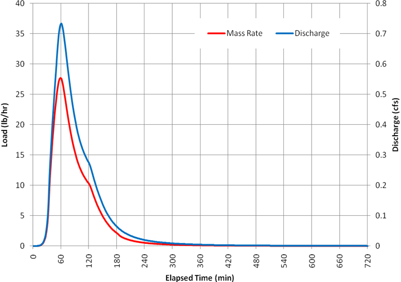
Figure 5‑6. Runoff flow and TSS load at site outlet for the 0.1 in. storm with EMC washoff

Exponential Washoff Results

Figure 5‑7 shows the simulated TSS concentration in the runoff from different Subcatchments using the 0.1 in. storm and the Exponential washoff equation. Unlike the EMC results, these concentrations vary throughout the runoff event and depend on both the runoff rate and the pollutant mass remaining on the Subcatchment surface. Figure 5‑8 shows the same plots but for the 0.23 in storm. Note two significant differences with respect to the results obtained for the 0.1 in storm. The maximum TSS concentrations are much larger (around 10 times) and the generation of TSS is much faster, as seen by the sharper-peaked pollutographs in Figure 5‑8. Finally, Figure 5‑9 shows the same graphs for the larger 1-in., 2-yr storm. The TSS concentrations are slightly larger than those for the 0.23 in. storm but the difference is much smaller than the difference between the 0.1 in and 0.23 in storms. Similar results hold for the pollutographs generated for the watershed’s outlet as seen in Figure 5‑10.

Figure 5‑7. TSS concentrations for the 0.1 in. storm with Exponential washoff

Figure 5‑8. TSS concentrations for the 0.23 storm with Exponential washoff

Figure 5‑9. TSS concentrations for the 2-yr (1 in.) storm with Exponential washoff

Figure 5‑10. TSS concentration at the site outlet for Exponential washoff

Even though the EMC and Exponential washoff models utilize different coefficients that are not directly comparable, it is interesting to compute what the average event concentration in the runoff from each Subcatchment was under the two models. The resulting averages are shown in Table 5‑6 for the case of the 0.23 in. storm. The point being made here is that even though the pollutographs produced by the two models can look very different, with the proper choice of coefficients it is possible to get event average concentrations that look similar. Although the results of the Exponential model are more pleasing to one’s sense of how pollutants are washed off the watershed, in the absence of field measurements one cannot claim that they are necessarily more accurate. Most H2OMAP SWMM modelers tend to use the EMC method unless data are available to estimate and calibrate the coefficients required of a more sophisticated buildup and washoff model.

Table 5‑6. Average TSS concentration for the 0.23 in. event

Subcatchment	EMC Model (mg/L)	Exponential Model (mg/L)
S1	170	180.4
S2	199.2	163.6
S3	117.2	67.7
S4	131.2	91.4
S7	0	0

5.5 Summary

This example illustrated how H2OMAP SWMM is used to model the quality of stormwater runoff within an urban catchment without any source or regional BMP controls. One pollutant, TSS, was simulated with one buildup method (exponential) and two different washoff methods (EMC and exponential). The key points illustrated in this example were:

1. H2OMAP SWMM models runoff water quality through the definition of pollutants, land uses, pollutant buildup, and pollutant washoff. Any number of user-defined pollutants and land uses can be modeled. Pollutant buildup and washoff parameters are defined for each land use and more than one land use can be assigned to each Subcatchment.

2. 2. There are several options available to simulate both pollutant buildup and washoff. Buildup expressions are defined by a buildup rate and a maximum buildup possible per unit of area or curb length. Pollutant washoff can be defined through an event mean concentration (EMC), a rating curve, or an exponential function. The exponential method is the only one that directly depends on the amount of buildup remaining on the surface. Rating-curve calculations are dependant only on the runoff across the Subcatchment, while EMCs have constant concentrations throughout the simulation.

3. 3. Exponential washoff produces a runoff pollutograph with rising and falling limbs, similar to that of a runoff hydrograph. The EMC pollutograph is flat throughout the duration of the event.

4. 4. Small storms can have a high impact on receiving waters because they are more frequent and can still generate significant washoff concentrations.

There are many uncertainties associated with both the process representation and the data required to properly estimate, calibrate and validate a runoff water quality model. It is strongly recommended that modelers use site specific data whenever possible when building a runoff water quality model with H2OMAP SWMM.