Example 7. Dual Drainage Systems in InfoSWMM and InfoSWMM SA
The post-development model in Example 2 simulated simple hydraulic routing within a surface drainage system that employed open channels in the form of gutters and swales. The three hydraulic routing methods (Steady Flow, Kinematic Wave and Dynamic Wave) were introduced and their effects on the drainage system behavior shown. Example 7 will convert some of the open channels in Example 2 to parallel pipe and gutter systems. A series of storm sewer pipes placed below the existing swales will also be added to help drain the downstream section of the site’s park area. Both the 2-yr and 100-yr design storms will be used to size and analyze the performance of this expanded dual drainage system. Particular attention will be paid to the interaction between the below-ground storm sewer flows and the above-ground street flows that occurs during high rainfall events. See the accompanying ‘H2OMAP SWMM Applications.HSM’ model, scenario ‘EX7-DUAL_DRAINAGE’ (with ‘child’ and ‘grandchild’ scenarios) for a complete worked out solution.
7.1 Problem Statement
The objective of this example is to simulate the interaction between the minor and major drainage systems through the interconnection of part of their underground and surface sections. For frequent events the minor or “initial” system operates (Grigg, 1996); overland flows are conveyed by gutters and enter into the pipe system. For large events these pipes surcharge and flood, and the major system handles the flows (Grigg, 1996). In particular, the entire street (not only the gutters) becomes a conveyance element.
Figure 7‑1 shows the post-development layout of the site analyzed in Example 2 (refer to ‘EX2-POST’ ‘parent’, ‘child’ and ‘grandchild’ scenarios in ‘H2OMAP SWMM Applications.HSM’). Example 2 modeled the drainage system with open channels and culverts whose invert elevations were the same as the ground surface elevations found on the site contour map. A series of below ground pipes will be added to the site that share inlets with the open (surface) channel running through the park. Gutters will also be added to the upstream section of the study area. The cross sections of these gutters will be that of a typical street, representing the surface “channel” through which water would flow if the pipe system surcharged and flooded the street. Thus, in this example the pipes and flow in gutters represent the minor system, and the channel in the park and the flow in streets represent the major system. The pipe system will be sized for the 2-yr event and its behavior observed during the major storm (100-yr event).
7.2 System Representation
Example 2 introduced junction nodes and conduit links as the basic elements of a drainage network. An example of the parallel pipe and gutter conveyance arrangement that will be used in this example is shown in Figure 7‑2. It consists of a below-grade circular pipe connected to manhole junctions on either end, plus an above grade street and gutter channel also connected to the same two manhole junctions. The details of the gutter inlet and drop structures that make the actual connection with the manholes are not important for our purpose. The parameters needed to characterize this type of node-link arrangement are as follows:

Figure 7‑1. Post-development site with simple drainage system

Figure 7‑2. Parallel pipe and gutter conveyance
· Manhole Invert Elevation
The invert elevation of the manhole junction is the elevation of the bottom of the manhole relative to the model’s datum (such as mean sea level). The invert elevation establishes the junction’s vertical placement in the H2OMAP SWMM model.
· Manhole Maximum Depth
The maximum depth of the manhole junction is the distance from its invert to the ground surface elevation where street flooding would begin to occur. If this maximum depth is left set at zero, H2OMAP SWMM automatically uses the distance from the junction’s invert to the top of the highest connecting link, which would be the top of the gutter/street channel in this particular example.
· Surcharge Depth
The surcharge depth of a junction is the additional depth of water beyond the maximum depth that is allowed before the junction floods. H2OMAP SWMM uses this depth to simulate pressurized conditions at bolted manhole covers or force main connections but it will not be used in this example. Different types of surcharge will be discussed later in this example.
· Conduit Offsets
The inlet offset for a conduit is the distance that its inlet end lies above the invert of the junction that it connects to. A similar definition applies to the offset for the outlet end of a conduit. In the parallel pipe and gutter system, the elevations of the gutters are set above the pipes using their inlet and outlet offsets (Figure 7‑2).
Note that because this representation of a dual drainage system has more than one conduit exiting a junction node, Dynamic Wave flow routing must be used to analyze it hydraulic behavior. An alternative way to represent these systems is to use the Overflow variety of Flow Divider nodes to connect pairs of pipes and gutter channels together. This scheme can be analyzed using the simpler Kinematic Wave method, where any flow in excess of the sewer pipe capacity would be automatically diverted to the gutter channel. The disadvantage of this approach is that cannot model a two-way connection between the pipes and gutters/streets, nor can it represent the pressurized flow, reverse flow and backwater conditions that can exist in these systems during major storm events.
Drainage System Criteria
The general drainage system criteria that will be used in this example are listed below. These criteria are based on those defined for the city of Fort Collins (City of Fort Collins, 1984 and 1997). Figure 7‑3 shows the different elements of the street considered in these criteria. Two storms will be used to design the drainage system: a minor or initial storm (2-yr) and a major storm (100-yr). The initial storm is one that occurs at fairly regular intervals while the major storm is an infrequent event. In this example, the streets are classified as “collectors”. Note that the general drainage criteria presented here apply only to this example and will change depending on the location of the system being designed. The criteria are:
· The minimum gutter grade (SL in Figure 7‑3) shall be 0.4%, and the maximum shall be such that the average flow velocity does not exceed 10 ft/sec.
· The cross-slope (Sx in Figure 7‑3) of all streets will be between 2% and 4%.
· The encroachment of gutter flows onto the streets for the initial storm runoff will not exceed the specification presented in the second column from the left in Table 7‑1. The encroachment of gutter flows on the streets for the major storm runoff will not exceed the specification presented in the third column from the left in Table 7‑1.
· The pipe system should carry the 2-yr storm and work as an open channel system.

Figure 7‑3. Elements of streets defined in the drainage criteria
Table 7‑1. General drainage system criteria for Fort Collins (City of Fort Collins, 1984 and 1997)
| Street Classification | Initial Storm | Major Storm |
| Local (includes places, alleys and marginal access) | No curb-topping. Flow may spread to crown of street | Residential dwelling and other dwelling cannot be inundated at the ground line. The depth of water over the crown cannot exceed 6 inches. |
| Collector | No curb-topping. Flow spread must leave at least one lane width free of water | Residential dwelling and other dwelling cannot be inundated at the ground line. The depth of water over the crown cannot exceed 6 inches. The depth of water over the gutter flowline cannot exceed 18 inches. (The most restrictive of the last two conditions governs) |
| Major Arterial | No curb-topptin. Flow spread must leave at least one-half of the roadway width free of water in each direction | Residential dwelling and other dwelling cannot be inundated at the ground line. The street flow cannot overtop the crown. The depth of water over the gutter flowline cannot exceed 18 inches (The most restrictive of the last two conditions governs) |
7.3 Model Setup
Figure 7‑4 shows the layout of the dual drainage system with the pipes, streets and swales that will be included in the model. Note that runoff from Subcatchments S1 and S2 is introduced first to the street system (gutters) through nodes Aux1 and Aux2, and then enters the storm sewers through inlet grates represented by nodes J1 and J2a. For the rest of the system the runoff is assumed to enter directly into the pipe system. The following steps are used to build the complete dual drainage model starting from the layout defined in the scenario ‘EX2-POST’ (see ‘EX2-POST’ ‘parent’, ‘child’ and ‘grandchild’ scenarios in ‘H2OMAP SWMM Applications.HSM’). The resulting scenario is ‘EX7-DUAL_ DRAINAGE_INITIAL’ (see ‘EX7-DUAL_DRAINAGE_INITIAL’ ‘child’ and ‘grandchild’ scenarios in ‘H2OMAP SWMM Applications.HSM’).
Surface Elements
1. The first step is to add the additional junction nodes Aux1, Aux2 and J2a, shown in Figure 7-4. The invert elevations of these nodes for now are simply their surface elevations (Aux1 = 4975 ft, Aux2 = 4971.8 ft, and J2a = 4970.7 ft).
2. Next the additional gutters C_Aux1, C_Aux1to2, C_Aux2, and C2a are added into the model and their lengths are determined using the Auto-Length option. These gutters have a roughness coefficient of 0.016.
3. Instead of the trapezoidal cross section used in Example 2, irregular shapes will be used to represent the cross sections of the gutter conduits. The transects that define these shapes are created using H2OMAP SWMM’s Transect Editor (see “Transects” in the Methodology section of the H2OMAP SWMM Users Guide). The transect Full_Street shown in Figure 7‑5 is used to represent the entire section of all streets within the study area. A cross-slope Sx = 4% is used to define this section. The transect Half_Street depicts only half of the Full_Street section, from the sidewalk to the crown of the street. It is used to represent the north-south street that runs down the east side of the development because its crown is considered to be the boundary of the catchment. The station and elevation data for both cross sections are listed in Table 7‑2.
4. The two types of transect cross-sections just created are then assigned to the corresponding street conduits shown in Figure 7‑4. Conduits C_Aux1, C_Aux1to2, and C_Aux2represent streets that have the Full_Street section. C2a and C2 represent streets that have the Half_Street section.
Table 7‑2. Cross-section data for street transects
| Full | Station | -40 | -20 | -20 | 0 | 20 | 20 | 40 |
| Street | Elevation | 1.3 | 0.5 | 0 | 0.8 | 0 | 0.5 | 1.3 |
| Half- | Station | -40 | -20 | -20 | 0 | 0 | - | - |
| Street | Elevation | 1.3 | 0.5 | 0 | 0.8 | 1.3 | - | - |

Figure 7‑4. Three-dimensional layout of the site's dual-drainage system

Figure 7‑5. FULL_STREET cross-section. The HALF_STREET section is half of this section.
Below-Ground Elements
The changes made so far have been to surface elements of the watershed. Now the pipes below the streets will be added to the drainage system and the invert elevations of the surface conduits will be re-defined.
1. Conduit C1 is replaced with a pipe (P1) and two pipes are added between nodes J2a and J2 (pipe P2) and J2 and J11 (pipe P3). The roughness of these three pipes is 0.016 and their diameter is 1 ft. As usual, the lengths of the pipes are calculated automatically with the Auto-Length tool.
2. At this point there are pairs of parallel links connected to the same input and output nodes (for example C2a and P2; C2 and P3). Right now, they are located at the same elevation (the surface elevation). These elevations must be adjusted so that the subsurface pipes lie below the surface gutters. This is done by decreasing the invert elevation of J1 and J5 by 4 ft (J1 = 4969 ft and J5 = 4965.8 ft), and raising the outlet offset of C_Aux1 to 4 ft and the inlet offset of C_Aux1to2 to 4 ft. Then, the invert elevations of J2a and J2 are decreased by 4 ft (J2a = 4966.7 ft and J2 = 4965 ft), an outlet offset of 4 ft is given to C_Aux2, an inlet and outlet offset of 4 ft is given to C2a, and an inlet offset of 4 ft and outlet offset of 6 ft to C2.
3. The properties of the different elements of the model should be those listed in Table 7‑3 and Table 7‑4. Table 7‑3 summarizes the junction inverts; Table 7‑4 shows the conduit shapes and their inlet and outlet offsets.
Park Area Elements
The next phase is to add the series of pipes that drain the park area containing the natural channel swales, shown in Figure 7-4. This process consists of the following steps.
1. A new node, Aux3, is added to the model with an invert elevation of 4974.5 ft. A new swale, C_Aux3, is defined connecting nodes Aux3 and J3. Its roughness is 0.05 and its cross section is the same as the cross section used in Example 2 for swales (for instance, the cross section of conduit C4).
2. Next the series of pipes that drain the park area is created as shown in Figure 7‑4. These pipes (P4, P5, P6, P7 and P8) connect with the surface system at junctions Aux3, J4, J5, J7, J10, and J11. The latter represent inlet grate structures in the surface swales. The roughness coefficient of these pipes is 0.016.
3. The pipes underneath the park have an initial diameter of 3 ft and lie 6 ft below the invert elevation of the natural channel through the park. These pipes are 2 ft deeper than the pipes buried below the streets to avoid giving P5 an adverse slope. The junctions where the swales and the pipe system connect together are assigned invert elevations that are 6 ft below the ground surface. The invert elevations of these junctions (in feet) become: Aux3 = 4968.5, J4 = 4965, J7 = 4963.5, J10 = 4957.8, J11 = 4957 and O1 = 4956.
4. As currently defined, one pipe in the model, P6, has an adverse slope. This negative slope is corrected by lowering the invert elevation of J7 from 6 ft below the surface to 8 ft (elevation J7 = 4963.5 ft).
5. The next step is to set the inlet and outlet offsets of the surface conduits where they share nodes with the series of pipes to maintain their surface elevations. The inlet and outlet offset elevations of C_Aux3, C4 and C10 are 6 ft and 0 ft, 6 ft and 4 ft, and 6 ft and 6 ft, respectively. Additionally, the inlet offset of C5 and C6 are increased to 4 ft and 8 ft respectively, and the outlet offset of C3 and C9 are increased both to 6 ft. These new offsets are defined to keep the swale at the surface. Note that the depths of the gutters are assumed negligible in this example. The depths of the swales (3 ft) are not considered negligible but were accounted for in Example 2 when their invert elevations were modeled.
6. The invert elevation of junctions J3, J6, J8 and J9 defined in Example 2 remain the same for this example. The final layout should look like the one shown in Figure 7‑6. The final invert elevations of the junctions as well as the size, inlet and outlet offsets of the conduits are summarized in Table 7‑3 and Table 7‑4.
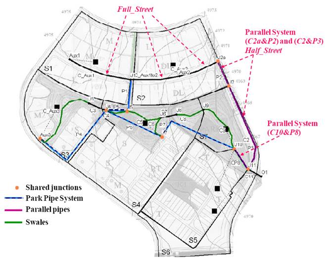
Figure 7‑6. Post-development site with dual drainage system
Table 7‑3. Junction invert elevations for dual-drainage system
| Junction ID | Surface Elevation (ft) | Elev. Change for Parallel Pipe (ft) | Final Invert Elevation (ft) |
| J1 | 4973.0 | 4 | 4969.0 |
| J2A | 4970.7 | 4 | 4966.7 |
| J2 | 4969.0 | 4 | 4965.0 |
| J3 | 4973.0 | 0 | 4973.0 |
| J4 | 4971.0 | 6 | 4965.0 |
| J5 | 4969.8 | 4 | 4965.8 |
| J6 | 4969.0 | 0 | 4969.0 |
| J7 | 4971.5 | 8 | 4963.5 |
| J8 | 4966.5 | 0 | 4966.5 |
| J9 | 4964.8 | 0 | 4964.8 |
| J10 | 4963.8 | 6 | 4957.8 |
| J11 | 4963.0 | 6 | 4957.0 |
| AUX1 | 4975.0 | 0 | 4975.0 |
| AUX2 | 4971.8 | 0 | 4971.8 |
| AUX3 | 4974.5 | 6 | 4968.5 |
| O1 | 4962.0 | 6 | 4956.0 |
Table 7‑4. Conduit shapes and offsets for dual-drainage
| Conduit ID | Type | Initial Depth or Diameter (ft) | Length (ft) | Inlet Offset (ft) | Outlet Offset (ft) |
| C2A | Half_Street | 1.3 | 157.48 | 4 | 4 |
| C2 | Half_Street | 1.3 | 526.00 | 4 | 6 |
| C3 | Culvert | 2.25 | 109.00 | 0 | 6 |
| C4 | Swale | 3.0 | 133.00 | 6 | 4 |
| C5 | Swale | 3.0 | 207.00 | 4 | 0 |
| C6 | Swale | 3.0 | 140.00 | 8 | 0 |
| C7 | Culvert | 3.5 | 95.00 | 0 | 0 |
| C8 | Swale | 3.0 | 166.00 | 0 | 0 |
| C9 | Swale | 3.0 | 320.00 | 0 | 6 |
| C10 | Swale | 3.0 | 145.00 | 6 | 6 |
| C11 | Culvert | 4.75 | 89.00 | 0 | 0 |
| C_AUX1 | Full_Street | 1.3 | 377.31 | 0 | 4 |
| C_AUX2 | Full_Street | 1.3 | 239.41 | 0 | 4 |
| C_AUX1TO2 | Full_Street | 1.3 | 286.06 | 4 | 0 |
| C_AUX3 | Swale | 3.0 | 444.75 | 6 | 0 |
| P1 | Pipe | 1.0 | 185.39 | 0 | 0 |
| P2 | Parallel Pipe | 1.0 | 157.48 | 0 | 0 |
| P3 | Parallel Pipe | 1.0 | 529.22 | 0 | 0 |
| P4 | Pipe | 3.0 | 567.19 | 0 | 0 |
| P5 | Pipe | 3.0 | 125.98 | 0 | 0 |
| P6 | Pipe | 3.0 | 360.39 | 0 | 0 |
| P7 | Pipe | 3.0 | 507.76 | 0 | 0 |
| P8 | Parallel Pipe | 3.0 | 144.50 | 0 | 0 |
7.4 Model Results
General System Behavior
The first step in analyzing this dual drainage system is to run the model in its preliminary sized state for the 2-yr storm with Dynamic Wave routing to check its general performance. The hyetographs for both the 2-yr and 100-yr storms are the same as those used in Example 1. For this run the reporting and wet-weather time steps were set to 1 minute, the routing time step to 15 seconds and the dry-weather runoff time step to 1 hour. The scenario for this initial system design is EX7-DUAL_ DRAINAGE_INITIAL (see ‘EX7-DUAL_DRAINAGE_INITIAL’ ‘child’ and ‘grandchild’ scenarios in ‘H2OMAP SWMM Applications.HSM’).
After running this scenario, the resulting Junction Summary report shows that no nodes are either surcharged or flooded. However, conduits P1, P2, and P3 were all surcharged (see the Max. Flow/Full Flow field in the Conduit Summary report) indicating that the system was undersized.
The differences in these reports illustrate that node surcharge and conduit surcharge are two different behaviors. Figure 7‑7 shows several examples of surcharge and flooding. Figure 7‑7a shows conduit surcharge; Figure 7‑7b shows conduit surcharge, node surcharge and node flooding; Figure 7-7c shows conduit surcharge and node surcharge; and Figure 7‑7d shows conduit surcharge, node surcharge and node flooding. Note that in the case of the open channel (Figure 7‑7a and Figure 7‑7b) node surcharge occurs simultaneously with node flooding.

Figure 7‑7. Examples of surcharge and flooding
The drainage criteria in Section 7.3 also require a minimum gutter grade of 0.4% and maximum average flow velocity of 10 ft/sec. Therefore, it is required to check that the minimum slope of the conduits representing gutters is larger than 0.4%. Table 7‑5, taken from the Conduit Report, shows the slopes of the conduits representing the gutters. All the gutters have a longitudinal grade of 0.4% or greater and thus meet the design standards considered for this example. The velocities in the gutters and all the conduits will be checked once the pipes of the system are properly sized.
Table 7‑5. Calculated gutter grades
| Conduit ID | Length (ft) | Slope (%) |
| C2A | 160 | 1.1 |
| C2 | 526 | 1.1 |
| C_AUX1 | 389 | 0.5 |
| C_AUX2 | 240 | 0.5 |
| C_AUX1TO2 | 276 | 0.4 |
Design for the 2-yr Storm
The next step of the analysis is to size the pipes so that they can carry the 2-yr storm without surcharging. In addition, the design criteria listed in Section 7.3 require the collector streets to be sized so there is no curb topping and at least one lane remains free of water. This phase of the analysis is carried out as follows:
1. The sizes of the pipes are iteratively modified, and the model run, until the Conduit Summary shows that no conduits are surcharged and that the values of the Max/Full Depthratio are close to 0.85 for all the pipes (a safety factor of 15% is considered to reduce the risk of surcharging). Table 7‑6 lists the standard pipe sizes that were used in this process. Table 7‑7 shows the results from three iterations, including the final one. Note how increasing the size of the upstream pipes allows some of the downstream pipes to be reduced in size (but made no smaller than the upstream ones).
2. Using the final pipe sizing from the previous step (Trial 3 in Table 7-6), the peak velocities in the conduits representing the streets are checked in the Conduit Summary. The peak velocity for all these conduits is less than 10 ft/sec, the maximum allowed by the drainage criteria.
3. According to the drainage criteria, no curb-topping should occur for the minor storm in any street. Figure 7‑5 shows that curb-topping implies a Max/Full Depth ratio of 0.5/1.3 = 0.38. The Conduit Summary for the final pipe sizing shows that the highest value of the Max/Full Depth ratio for the street conduits is 0.29 for conduit C_Aux2. Thus, the final design of the system is appropriate in terms of the flows in the streets.
The scenario with the final pipe sizes for this example is ‘EX7-DUAL_DRAINAGE_FINAL’ (see ‘EX7-DUAL_DRAINAGE_FINAL’ ‘child’ and ‘grandchild’ scenarios in ‘H2OMAP SWMM Applications.HSM’).
Table 7‑6. Available drainage pipe sizes
| in. | ft | in. | ft | in. | ft | in. | ft |
| 6 | 0.5 | 18 | 1.5 | 24 | 2.0 | 38 | 3.2 |
| 12 | 1.0 | 20 | 1.7 | 28 | 2.3 | 42 | 3.5 |
| 16 | 1.3 | 22 | 1.8 | 36 | 3.0 | 48 | 4.0 |
Table 7‑7. Iterations for 2-yr storm pipe sizing
| Pipe | Trial 1 | Trial 2 | Trial 3 | ||||||
| Size (ft) | Surcharged | Max/Full Depth | Size (ft) | Surcharged | Max/Full depth | Size (ft) | Surcharged | Max/Full Depth | |
| P1 | 1 | yes | 0.85 | 1.3 | no | 0.69 | 1.3 | no | 0.71 |
| P2 | 1 | yes | 1.00 | 1.3 | yes | 0.90 | 1.5 | no | 0.67 |
| P3 | 1 | yes | 1.00 | 1.3 | no | 0.90 | 1.5 | no | 0.80 |
| P4 | 3 | yes | 0.27 | 2.0 | no | 0.52 | 1.7 | no | 0.64 |
| P5 | 3 | no | 0.29 | 2.0 | no | 0.58 | 1.8 | no | 0.65 |
| P6 | 3 | no | 0.36 | 2.0 | no | 0.71 | 2.0 | no | 0.72 |
| P7 | 3 | no | 0.48 | 2.0 | no | 0.81 | 2.0 | no | 0.81 |
| P8 | 3 | no | 0.53 | 3.2 | no | 0.51 | 3.2 | no | 0.51 |
Major Storm Performance
Finally, the model is run for the 100-yr storm by changing to the ‘EX7-DUAL_DRAINAGE_FINAL_100YR’ scenario (see the ‘EX7-DUAL_DRAINAGE_FINAL_ 100YR’ scenario in ‘H2OMAP SWMM Applications.HSM’). The Junction Summary report shows that no nodes are surcharged or flooded during the 100-yr storm. Additionally, the Conduit Summary shows that, as expected, all of the pipes are surcharged. According to the Conduit Summary table, the highest velocities occur in conduits C7, C11 and P8 (11.29, 11.90 and 10.70 ft/sec respectively), all of them over 10 ft/sec. Standard drainage criteria define a maximum allowable velocity in pipes and culverts of 15 to 18 ft/sec (CCRFCD, 1999; Douglas County, 2008). Thus, the maximum velocities predicted for pipe P8 and culverts C7 and C11 are acceptable, and no re-sizing of the conveyance system is required. Finally, the Conduit Summary table shows that the Max/Full Depth value of all street conduits is less than one. Therefore the water depth in the streets never reaches the crown or the highest point of the sidewalks, and the requirements for the 100-yr storm are successfully satisfied.
To illustrate the complex flow conditions that can occur in these systems, Figure 7‑8 shows the hydrographs in pipes P5 and P6 under the 100-yr storm. Negative flows caused by backwater effects occur in both pipes after 30 minutes of simulation. These special flow conditions can be only simulated when Dynamic Wave routing is used, which demonstrates the capabilities of this method. These negative discharges do not occur for the 2-yr storm. This shows that the behavior of a system under a minor and a major event can be quite different. In this case, the runoff generated by Subcatchment S4 into junction J7 for the 100-yr storm is large enough to cause a backwater effect that generates these negative flows.

Figure 7‑8. Flows in pipes P5 and P6 during the 100-yr storm
Another way to visualize the behavior of the dual drainage system is with Profile Plots. Figure 7‑9 contains two such plots stacked on top of one another. They depict the surcharge condition that occurs between nodes J2a, J2, and J11 at 34 minutes into the 100-yr storm. The lower plot applies to the below-ground sewer pipes P2 and P3 and shows that both pipes are surcharged. The upper plot is for the streets C2a and C2 that lie above P2 and P3. The water levels at junctions J2a and J2 are high enough to cause water to flow out of the sewer pipe P2 and onto the street, but not high enough to flood the street. On the other hand, the invert elevation of junction J11 is low enough so that the surcharged pipe P3 does not create street flooding and instead, street flow re-enters the sewer system there. (The plot makes it appear that the flow at the downstream end of street C2 is zero, but this is just an artifact of the way that H2OMAP SWMM draws the water surface profile within a conduit (by connecting the water elevations between its end nodes without allowing the profile to cross either its bottom or top surface)).
7.5 Summary
This example built on the simple drainage system modeled in Example 2. It converted some of the open surface channels used in that example to parallel pipe and gutter systems and added a new series of pipes to drain the downstream section of the park. The system was sized for a minor (2-yr) storm event and its behavior was also analyzed under a major (100-yr) storm event. The key points illustrated in this example were:


Figure 7‑9. Surcharge behavior along the eastern boundary of the site
1. The three-dimensional structure of dual drainage systems can be modeled by using manhole junctions set below ground that connect parallel pairs of sewer pipes and gutter/street channels, where the latter are offset to ground elevation.
2. These systems are designed so that the below-ground sewer system will flow only partly full during the more frequent minor storm events and will surcharge into the street channels during the larger, less frequent major events without causing any overtopping of the street.
3. An iterative process can be used to properly size the sewer pipe elements to meet both the small storm and large storm design criteria.
4. Most of the results needed to evaluate the performance of a dual drainage system can be found in H2OMAP SWMM’s Junction Summary and Conduit Summary tables.
As this example shows, dual drainage system models require a significant amount of additional effort to set up. The need to represent both the minor and major portions of a drainage system will depend on the objectives set forth for the analysis and on the level of detail required from the model.