Example 10. LID Controls in InfoSWMM and InfoSWMM SA

Example 10. LID Controls in InfoSWMM and InfoSWMM SA

This example demonstrates how to model two Low Impact Development (LID) control alternatives, filter strips and infiltration trenches. The detention pond modeled in Example 3 is an example of a subdivision-scale drainage control structure. The LIDs in this example are hydrologic source controls that operate on a smaller scale and rely heavily on infiltration and distributed small-scale storage to reduce the overall runoff volume from a watershed and control water quality. This section uses the newer SWMM 5 LID Controls.

InfoSWMM H2OMap SWMM InfoSWMM SA is better suited to simulating some types of hydrologic source control techniques than others. Filter strips and infiltration trenches are two such source controls. This example will illustrate how they can be represented in InfoSWMM H2OMap SWMM InfoSWMM SA by applying them to the same catchment area studied in the previous Examples 1, 2 and 3.

4.1 Problem Statement

In Examples 1 and 2, runoff estimates for the 29 acre residential development shown in Figure 4-1 were made without any source controls in place. In this example, the effects that infiltration trenches (IT) and filter strips (FS), two commonly used LIDs, have on the site’s runoff will be examined. As illustrated in Figure 4-1, four infiltration trenches will be placed at each side of the east-west street in the upper part of the study area. Additionally, filter strips will be used to control the runoff from lots S, M and M2, located in the southwest section of the site. These strips will be built along the sidewalks so they control runoff from the lots before it reaches the gutters.

In Example 3 the quantitative objective for the design of a detention pond was to reduce the post-development watershed discharge to pre-development levels. The LIDs modeled here will not be designed to accomplish a specific quantitative objective but rather to achieve a general reduction in runoff volume to help meet sustainability goals and place a lower burden on stormwater controls further downstream in the basin. The performance of the LIDs for the 2-, 10- and 100-yr storms will be analyzed.

4.2 System Representation

The two LIDs modeled here are filter strips and infiltration trenches. Guidance in the representation of these and other LIDs can be found in Huber at al. (2006).

Figure 4-1. Post-development site with LIDs in place

Filter Strips

Filter strips are grassed or vegetative areas through which runoff passes as sheet flow. They do not effectively reduce peak discharges but are effective in removing particulate pollutants for small storms (< 1 year storm) (Akan and Houghtalen, 2003). Flat slopes (<5%) and low to fair permeability (0.15 to 4.3 mm/h or 0.006 to 0.17 in/h) of natural subsoil are required for their effective operation (Sansalone and Hird, 2003). InfoSWMM H2OMap SWMM InfoSWMM SA does not have a unique visual object to represent filter strips but they can be represented as a pervious Subcatchment that receives runoff from an upstream Subcatchment as illustrated in Figure 4-2. The two most important processes that must be simulated with filter strips are infiltration and storage. A filter strip can be simulated as a 100% pervious Subcatchment whose geometry (area, width and slope) is obtained directly from the field. This Subcatchment receives water from an upstream contributing area (impervious or semi-impervious) and drains to a conduit representing the gutter or street. The infiltration for a filter strip can be simulated using any of InfoSWMM H2OMap SWMM InfoSWMM SA infiltration options.

Figure 4-2. Schematic representation of a filter strip

Infiltration Trenches

Infiltration trenches are excavations backfilled with stone aggregate used to capture runoff and infiltrate it to the ground (Guo, 2001). Subsoil with a minimum permeability of 13 mm/h (0.5 in/h) is required for a good performance (U.S. EPA, 1999). The most important processes that must be simulated for an infiltration trench are infiltration, storage and the water flow along the trench. Figure 4-3 shows a workable InfoSWMM H2OMap SWMM InfoSWMM SA representation of an infiltration trench. It consists of a rectangular, fully pervious Subcatchment whose depression storage depth equals the equivalent depth of the pore space available within the trench.

Figure 4-3. Schematic representation of an infiltration trench

4.3 Model Setup – Filter Strips

Figure 4-1 shows the locations of the filter strips (FS) to be modeled in this example. The initial InfoSWMM H2OMap SWMM InfoSWMM SA scenario to which the LIDs will be added is EX2-POST, which includes both Subcatchments and a runoff conveyance system in it. Figure 4‑1 will be used as the backdrop of the new model to help facilitate the placement of the filter strips. The image file for this backdrop is named Site-Post-LID.jpg. Table 4‑1 lists the Subcatchment to which each filter strip belongs and the length of each strip.

Table 4-1. Subcatchments containing filter strips

Subcatchment Controlled	Filter Strip	Filter Strip Length (ft)
S3	FS 1	410
S3	FS 2	105
S3	FS 3	250
S4	FS 4	359
S4	FS 5	190
S4	FS 6	345
S3 and S4	FS 7	375

The filter strips to be constructed are identified in Table 4‑1 with letters FS and a number. In the model being built some of the strips will be aggregated together as they are represented as new Subcatchments. These filter-strip Subcatchments will be identified as “S_FS_number”.

To better estimate the runoff treated by the filter strips, Subcatchments S3 and S4 will be discretized further. S3 will be divided into three Subcatchments S3.1, S3.2 and S3.3 and S4into four Subcatchments S4.1, S4.2, S4.3 and S4.4 as shown in Figure 4‑4. It will be necessary to re-estimate the average overland runoff length and new Subcatchment widths, slopes and percents imperviousness to place in the model. Refer to Example 1 for help in determining the new Subcatchments’ hydrologic properties. The slopes of the new Subcatchments representing lots will be 2%. The same Horton infiltration rates already defined in the previous examples will be used here: 4.5 in/hr for the maximum, 0.2 in/hr for the minimum and 6.5 hr-1 for the decay constant. With the addition of these new Subcatchments and the re-discretization of some of the original ones, it is necessary to define new channels and junctions to connect them to the drainage system. These new elements are illustrated in Figure 4‑4 (pipes in red and junctions in blue). Table 4‑2 lists the properties of the new junctions and Table 4‑3 does the same for the new conduits.

Table 4‑4 summarizes the properties of the new Subcatchments. The outlets of the new Subcatchments (S3.2, S3.3, S4.2, and S4.3) are not junctions but filter strips represented as Subcatchments. This cascade layout used in the InfoSWMM model is shown in Figure 4‑5 for Subcatchments S3.1, S3.2 and Figure 4‑6 for Subcatchments S4.1, S4.2, S4.3 and S4.4.

The length of the filter strips (i.e., the overland flow length existing between lots and streets) will be 4 feet and the slope of each strip along this length is the same as the typical lot slope of 2%. The widths of the strips (perpendicular to the overland flow direction) is computed directly from the map with the Measure tool as explained in Example 1 and are given in the last column of Table 4‑5.

Table 4-2. Properties of the new junctions

New Junction	Invert Elevation (ft)
J15	4974.5
J16	4973.5
J17	4973.5

Table 4-3. Properties of the new conduits

New Conduit	Inlet Node	Outlet Node	Length (ft)	Type of Section1	Manning Coefficient	Maximum Depth (ft)	Bottom Width (ft)	Left Slope	Right Slope
C15	J15	J3	444.75	Swale	0.05	3.0	5	5	5
C16	J17	J5	200.16	Swale	0.05	3.0	5	5	5
C17	J16	J7	300.42	Gutter	0.016	1.5	0	0.0001	25
1Type of section based on sections defined in Example 2

Figure 4-4. Re-dicretization of Subcatchments S3 and S4

Table 4-4. Properties of the Subcatchments derived from S3 and S4

New Subcatchment	Outlet	Area (ac)	Width (ft)	Slope (%)	Imperviousness
S3.1	J3	1.29	614	4.7	0
S3.2	S_FS_1	1.02	349	2.0	65
S3.3	S_FS_2	1.38	489	2.0	58
S4.1	J6	1.65	580	5.0	0
S4.2	S_FS_3	0.79	268	2.0	70
S4.3	S_FS_4	1.91	657	2.0	65
S4.4	J9	2.40	839	2.0	69

Table 4-5. Widths of the filter strip Subcatchments

Filter Strip	Subcatchment Controlled	Composition	Partial Widths (ft)	Total Widths (ft)
S_FS_1	S3.2	FS 1	410	410
S_FS_2	S3.3	FS 2 + FS 3 + part FS 7	105 + 250 + 108	463
S_FS_3	S4.2	Part FS 7	267	267
S_FS_4	S4.3	FS 4 + FS 5 + FS 6	359 + 190 + 345	894

Figure 4‑5. Representation of Subcatchments S_FS_1, S3.1, and S3.2

Figure 4-6. Representation of Subcatchments S_FS_3, S_FS_4, S4.1, S4.2, and S4.3

Table 4-6 summarizes the characteristics of the Subcatchments used to model the filter strips in this example. The areas of the filter strips are calculated from the lengths of the strips measured in the model and the flow path length (4 ft) used in this example. This means the areas calculated by Auto-Length for these Subcatchments need to be replaced with those calculated in Table 4-6.

Table 4-6. Properties of the filter strip Subcatchments

Subcatchment	Upstream Subcatchment	Outlet	Area1 (ft2)	Area (ac)	Width2 (ft)	Slope (%)	Depression3 Storage (in)
S_FS_1	S3.2	J15	1640	0.038	410	2.0	0.3
S_FS_2	S3.3	J17	1852	0.043	463	2.0	0.3
S_FS_3	S4.2	J16	1068	0.025	267	2.0	0.3
S_FS_4	S4.3	J16	3576	0.082	894	2.0	0.3
1Area = length of the trench x 4 ft width perpendicular to the flow direction.
2Same width as adjacent Subcatchment.
3Same as pervious area depression storage of surrounding area.

Once the filter strip properties shown in Table 4-5 and Table 4-6 are added to the model, all filter strips are assigned a zero percent imperviousness, an impervious roughness of 0.015 and an impervious depression storage of 0.06 in (although neither of the latter properties are used due to 0% imperviousness); a pervious roughness of 0.24, and a pervious depression storage of 0.3 in. These last two values are the same as those for the rest of the pervious areas within the watershed. Finally, both the maximum and minimum infiltration rates for Horton infiltration are set to the same value, 0.2 in/hr, which is the minimum infiltration rate of the soil in the study area. This is a conservative approach that takes into account possible losses to infiltration capacity as well as the fact that soil may be saturated at the beginning of a new storm.

All Subcatchments must have a rain gage assigned to them in order for the InfoSWMM model to run. However, no rain should fall on the Subcatchments representing the filter strips because their areas are considered part of the Subcatchments within which they were placed. Thus, a new Time Series called “Null” is defined with a single time and rain value equal to zero. A new rain gage also called “Null” is created and linked to the time series “Null”. This gage is defined to be the rain gage of all the filter strip Subcatchments, while the Subcatchments that generate runoff are connected to the original rain gage “RainGage”, as in the previous examples.

4.4 Model Setup – Infiltration Trenches

The infiltration trenches (IT) included in this example are located in the north part of the study area (see Figure 4-1). To model these devices Subcatchments S1 and S2 are first divided into six smaller Subcatchments as shown in Figure 4-7. Their areas are determined automatically by using the InfoSWMM H2OMap SWMM InfoSWMM SA Auto-Area tool. Their widths are based on an assumed urban runoff length of 125 ft (measured from the back of the lot to the street), as discussed in Example 1. The imperviousness of each newly sub-divided Subcatchment is based on the type of land use (M, L or DL) as listed in Table 1-6 of Example 1. Table 4-7 summarizes the properties of the newly sub-divided Subcatchments. The remaining properties not shown in the table (Horton infiltration, pervious depression storage, etc.) are the same as those given to the original Subcatchments.

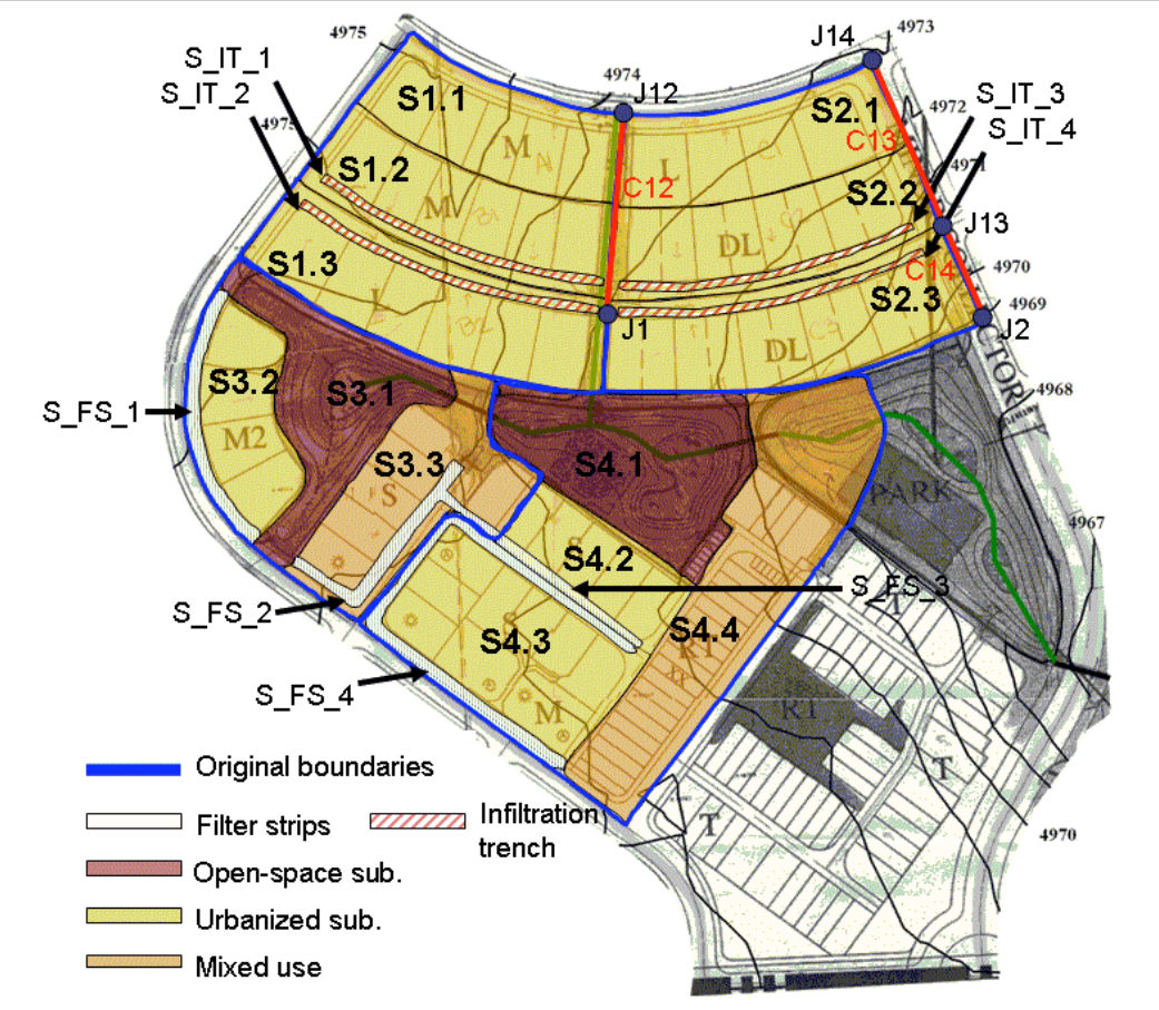
Figure 4-7. Re-discretization of Subcatchments S1 and S2 for infiltration trenches

Table 4-7. Properties of the Subcatchments derived from S1 and S2

New Subcatchment	Outlet	Area (ac)	Width (ft)	Slope (%)	Imperviousness
S1.1	J12	1.21	422	2.0	65
S1.2	S_IT_1	1.46	509	2.0	65
S1.3	S_IT_2	1.88	655	2.0	45
S2.1	J14	1.30	453	2.0	45
S2.2	S_IT_3	1.50	523	2.0	70
S2.3	S_IT_4	1.88	655	2.0	70

The infiltration trenches added to the model are identified in Table 4‑8. Their names begin with the letters IT followed by a number. The location of these infiltration trenches is shown in Figure 4-7. The four infiltration trenches are added into the model as Subcatchments and have an S_ prefix added to their name. They serve as the outlets of Subcatchments S1.2, S1.3, S2.2 and S2.3 as shown in Table 4‑9. The outlets of the other new Subcatchments, S1.1 and S2.1, are junctions J12 and J14, respectively.

When sizing the infiltration trenches, note that the definition of length and width is opposite of the manner in which length and width were defined for filter strips. The length of each infiltration trench is listed in Table 4-8. The trench area can be computed using this length and assuming a width of 3 ft. The widths and areas of each infiltration trench are listed in Table 4-9. Each trench is modeled as having a depression storage depth of 1.2 ft (below this depth water is infiltrated, while above this depth there is flow along the trench). The actual storage depth of the infiltration trenches is 3 ft, but when the 40% porosity of the 1-1/2 in. diameter gravel filling the trenches is considered, the depth of the trenches available to store the water to be infiltrated is reduced to 40% of the actual trench depth. Table 4-9 summarizes the properties assigned to the infiltration trench Subcatchments.

Table 4-8. Subcatchments containing infiltration trenches

Subcatchment Controlled	Infiltration Trench	Trench Length (ft)
S1	IT 1	450
S1	IT 2	474
S2	IT 3	450
S2	IT 4	470

Table 4-9. Properties of the infiltration trench Subcatchments

Subcatchment	Upstream Subcatchment	Outlet	Area1 (ft2)	Area (ac)	Width (ft)	Slope2 (%)	Depression3 Storage (in)
S_IT_1	S1.2	J1	1350	0.031	3.0	0.422	14.4
S_IT_2	S1.3	J1	1422	0.033	3.0	0.422	14.4
S_IT_3	S2.2	J13	1350	0.031	3.0	0.444	14.4
S_IT_4	S2.3	J13	1410	0.032	3.0	0.468	14.4
1Area = length of the trench x 3 ft width perpendicular to the flow direction.
2Slope as computed from the site map..
3This corresponds to the effective depth of the trench, 0.4 x 36 in.

The slopes of the infiltration trenches are calculated directly from the site map, their imperviousness is 0%, their Manning’s roughness coefficient is 0.24, and their storage depths are accounted for by setting their depression storage to the effective storage depth of 14.4 in (1.2 ft). As was done for the filter strips, a constant (minimum) soil infiltration capacity of 0.2 in/hr will be used for the infiltration trenches. This ignores any horizontal infiltration that might occur through the sides of the trench. Also the rain gage assigned to each trench Subcatchment is the newly created “Null” rain gage so that no rainfall occurs directly over the trench’s area.

This trench design assumes there is no barrier affecting the flow of water into the trench. A layer of grass and soil above the 1-1/2 in. diameter gravel, for example, might slow the rate of flow into the trench; causing a smaller quantity of flow to be treated by the trench. This will be touched on again in the results section of this example.

To complete the model it is necessary to define the additional channels and junctions that connect the newly added Subcatchments to the drainage system. These new elements are illustrated in Figure 4-7 (conduits in red and junctions in blue). Table 4-10 lists the properties of the new junctions and Table 4-11 does the same for the new conduits.

Table 4-10. Properties of the new junctions

New Junction	Invert Elevation (ft)
J12	4973.8
J13	4970.7
J14	4972.9

Table 4-11. Properties of the new conduits

New Conduit	Inlet Node	Outlet Node	Length (ft)	Type of Section1	Manning Coefficient	Maximum Depth (ft)	Bottom Width (ft)	Left Slope	Right Slope
C18	J12	J1	281.7	Swale	0.050	3.0	5	5	5
C13	J14	J13	275.5	Gutter	0.016	1.5	0	0.0001	25
C14	J13	J2	157.5	Gutter	0.016	1.5	0	0.0001	25
1Type of section based on sections defined in Example 2

4.5 Model Results

The final model with all LIDs included can be found in the EX4 scenario. It was run under Dynamic Wave flow routing using a wet runoff time step of 1 minute, a reporting time step of 1 minute, and a routing time step of 15 s for each of the three design storms. Figure 4-8 compares the resulting influent and effluent runoff hydrographs for filter strip S_FS_1 for each of the design storms. Figure 4-9 does the same for infiltration trench S_IT_1. Results for the other LIDs look similar to these. Table 4‑12 and Table 4-13 list runoff coefficients for each filter strip and infiltration trench, respectively. As used here, the runoff coefficient is the ratio of the effluent-runoff volume flowing out of the LID to the influent-runoff volume flowing into the LID. The fractional reduction in runoff volume provided by the LID is simply 1 minus the runoff coefficient.

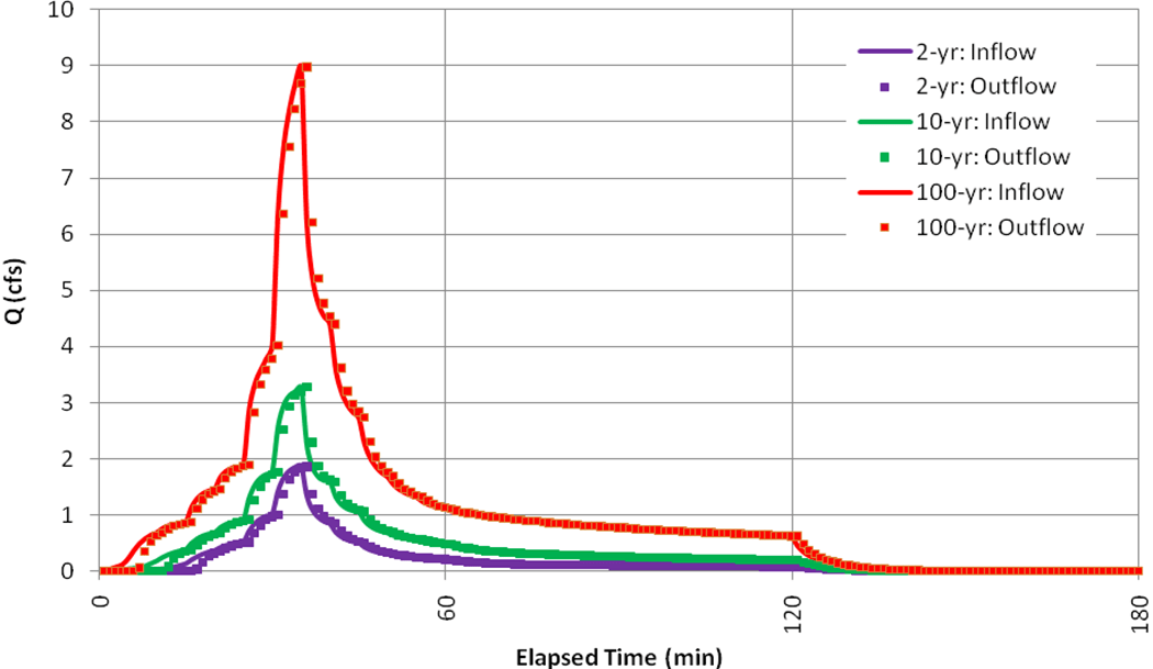
Figure 4-8. Influent and effluent hydrographs for filter strip S_FS_1

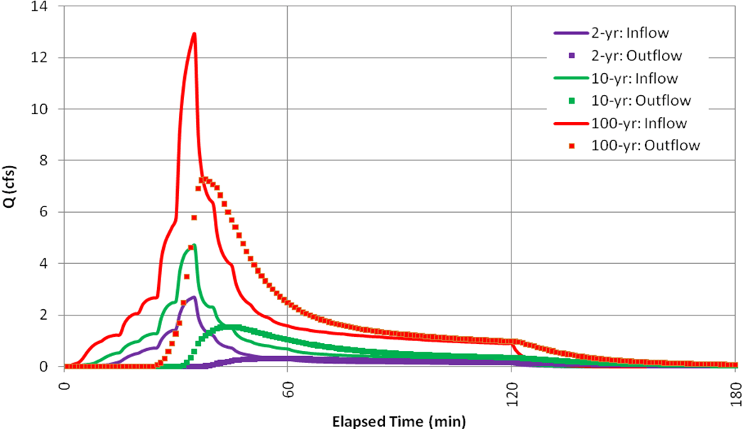
Figure 4-9. Influent and effluent hydrographs for infiltration trench S_IT_1

Table 4-12. Runoff coefficients for filter strips

Filter Strip	Runoff Coefficient
	2-year Storm	10-year Storm	100-year Storm
S_FS_1	0.95	0.98	0.99
S_FS_2	0.95	0.98	0.99
S_FS_3	0.96	0.98	0.99
S_FS_4	0.94	0.97	0.99

Table 4-13. Runoff coefficients for infiltration trenches

Infiltration Trench	Runoff Coefficient
	2-year Storm	10-year Storm	100-year Storm
S_IT_1	0.45	0.73	0.89
S_IT_2	0.35	0.71	0.90
S_IT_3	0.51	0.75	0.90
S_IT_4	0.59	0.79	0.92

It is apparent that filter strips provide negligible runoff control, with the outflow rate very nearly equaling the inflow rate for all storm magnitudes. This confirms what was mentioned in section 4.2 regarding the utility of filter strips, i.e. they are primarily pollutant removal devices and provide no benefit in controlling runoff flow rates or volumes. In contrast, all of the infiltration trenches provide significant reductions in runoff volume, particularly for the smaller rainfall events. It should be remembered, however, that the trenches in this example do not have grasses planted above the gravel backfill. Adding such a vegetative layer to the trench may reduce its effectiveness, depending on how it is designed.

Figure 4-10 compares the discharges simulated at the outlet of the study area for each design storm (2-, 10- and 100-yr return period) both with and without LIDs. For each design storm LIDs reduce both runoff volumes and peak discharges. As the storm event becomes larger, LIDs become less effective and the attenuation of their volumes and peak-discharges is reduced. These percent reductions in outlet volumes and peaks are compared in Figure 4‑11. It shows how the benefit of LID controls decrease with increasing size of storm.

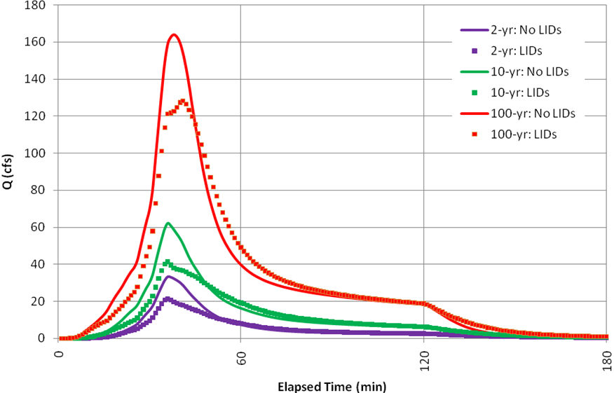
Figure 4-10. Comparison of outlet discharges with and without LID controls

Figure 4-11. Percent reduction in outlet peak flows and runoff volumes with LIDs

4.6 Alternative Routing Method (Sub-Area Routing)

An alternative method to modeling LIDs, other than creating additional Subcatchments as used in this example, is to use Sub-Area Routing. Each Subcatchment modeled in InfoSWMM is composed of two sub-areas, an impervious sub-area and a pervious sub-area, and optional parameters called Runoff Routing Destination and % of Runoff Routed to Destination which appear in the Attribute Browser.

Runoff Routing Destination has three options: Outlet, Impervious and Pervious. The Outlet option ((a) in Figure 4-12) routes the runoff from both sub-areas directly to the Subcatchment’s outlet. The Pervious option ((b) in Figure 4-12) routes the runoff from the impervious sub-area across the pervious sub-area and then to the outlet, and the Impervious option ((c) in Figure 4-12) routes the runoff from the pervious sub-area across the impervious sub-area and then to the outlet.

When the runoff from the impervious surface is routed across the pervious surface ((b) in Figure 4-12), some of the runoff is lost to infiltration and depression storage in the pervious sub-area. The graph below shows the typical effect on runoff these three sub-area routing methods have when applied to a single Subcatchment. Note that because the runoff produced by the pervious area in this case is negligible, the “100% routed to Outlet” and the “100% routed to Impervious” cases are practically the same.

Figure 4-12. Comparison of sub-area routing methods

The Sub-Area Routing - Pervious option can be used to model LIDs. This is done by representing the LID as the pervious sub-area, setting the Subcatchment’s pervious values to those of the LID, routing the runoff from the impervious subarea of the Subcatchment to the pervious subarea, and defining the Percent Routed to represent the percentage of impervious surface connected to the LID.

Modeling LIDs with this method implies that the entire Subcatchment’s pervious surface represents the LID. This approach is not as flexible as the one presented in this example because the slope and width of the LID must be those of the Subcatchment, which is not always the case.

4.7 Summary

This example illustrated how InfoSWMM H2OMap SWMM InfoSWMM SA can be used to evaluate two types of Low Impact Development (LID) alternatives, filter strips and infiltration trenches. The key points illustrated in this example were:

1. A filter strip can be modeled as a rectangular, 100% pervious Subcatchment with a constant infiltration rate.

2. An infiltration trench can be modeled as a rectangular, 100% pervious Subcatchment with a constant infiltration rate whose depression storage is the effective pore volume depth of the trench.

3. Modeling these types of LIDs can require a finer level of Subcatchment discretization to properly account for their localized placement.

4. Infiltration trenches (without a top soil layer) are more effective than filter strips in reducing runoff volumes and peaks.

5. The effectiveness of LIDs at reducing runoff volumes and peaks decreases with increasing size of storm event.

Although this example used a series of design storms to evaluate LID performance, a more accurate estimate of their stormwater control capabilities would require that a continuous long-term simulation be run for the site. Using several years’ worth of actual rainfall inputs would allow the model to properly account for the variation in antecedent soil conditions between storm events. This factor becomes a critical concern when infiltration-based controls are being considered. Example 9 in this manual illustrates how to perform such a continuous simulation.