Force Mains in InfoSewerForce Main Network Solution

The Force Main Network Solution allows the simulation of multiple upstream and downstream force mains entering and leaving one chamber junction during an Extended Period Dynamic Simulation or EPS solution in Sewer. All of the force mains, pumps, wet wells and force main chamber junctions that are connected are considered as one force main network in the EPS solution. You can have more than one force main network in a large Sewer model separated by gravity pipes and loading manholes. The individual force main networks are solved iteratively with different upstream head and downstream tail manholes which connect the force main network(s) to the rest of the network.

A force main network consists of the following elements:

• Wet well
• Pump
• Junction Chamber
• Head Manhole where flow from other parts of the sewer system enters the force main network
• Tail manhole where the flow leaves the force main network.

The head and tail manhole for one force main network is determined by the program based on the geometry of the network. The force main network starts at a wet well, includes the pumps connecting the wet well to the force main links and also includes the actual force main links and force main connecting junction chambers. You can also connect a force main to the gravity mains without an intermediate wet well and pump(s).

The boundary conditions of the force main network are:

• Water heads at the wet wells which vary according to the inflow from the upstream sections of the sewer network and outflow to the force main network
• Water head at the tail manholes which are calculated as the maximum discharge head (invert + diameter) of all the force mains that end at that manhole. Water entering the tail manholes will be routed downstream after the force main network flows are calculated.

For example, assuming there are n1 wet wells, n2 head manholes, n3 tail manholes, n4 junction chambers and p1 pumps and p2 force mains, the program must solve the network hydraulics to get n2+n4 water head values and p1+p2 flow values iteratively using the Newton-Raphson method. The solution iterates until the mass and energy of the force main network is in balance.

The hydraulic equations used in the solution are:

• Head/Flow relationship of the force mains and pumps (p1+p2 equations)
• Mass balance at head nodes and junction chambers (n2+n4 equations)

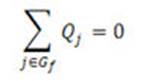
For head nodes, water entering the network from other sections of the sewer system must equal the flow sum of force mains that connect to it:

Where Q = Flow; Gv = group of gravity pipes connecting to the head manhole; and Gf = group of force mains connecting to the head manhole. The sum of the gravity flow into the wet well or head manholes is balanced by the sum or flow out of the force main network in the force main pipes.

For junction chambers, which are connected to only force main pipes:

For force mains, Hazen-Williams equation describes the flow/head loss relationship within a force main. The flow out of and the flow into the junction chamber is in balance. The head at the junction manhole is iterated until the flows are in balance.

For pumps that are neither Inflow Control nor Discharge Control, the pump curve is used to estimate the flow and head gain relationship within a pump. For Inflow Control and Discharge Control pump, pump flow as control values are fixed and the equation Q = Qcontrol, where Qcontrol is the controlling pump value. For such situations, the pump is actually modeled as variable speed pump and pump speed will be calculated with Newton-Raphson method to achieve the flow control objective.

Force Main Graph

Displays simulation results for one force main. The graph X-axis displays time in units defined with the Simulation Time command (Report Timestep) and the Y-axis displays simulation results for the selected force main. Upon choosing this graph type you are prompted to choose a force main. Upon choosing this graph type, you are prompted to choose a force main. Once selected, the graph appears in the Output Report Manager window. Gravity main graphs can display the flow, velocity, headloss for the force main and the water quality concentration (if simulated).

Extended Period Dynamic Simulation (Unsteady Flow)

InfoSewerH20Map Sewer Pro tracks the movement of wastewater flowing through the network over an extended period of time under varying wastewater loading and operating conditions. The extended period simulation (EPS) model implemented in InfoSewerH20Map Sewer Pro is a fully dynamic (unsteady) model and is predicated on solving a simplified form of the full 1D Saint-Venant equations neglecting local acceleration.

The Saint-Venant equations or full dynamic wave equations for open channel flow routing consist of the conservation of momentum equation and the equation of continuity. The momentum equation is:

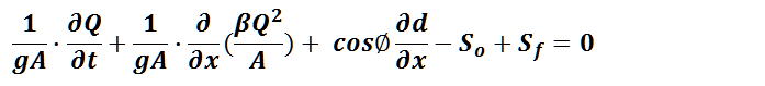
The continuity (mass conservation) equation is:

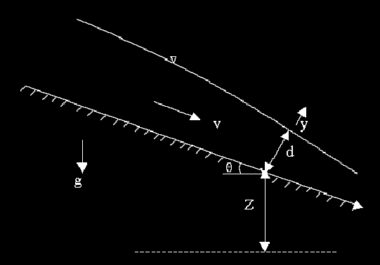
where

x = distance along the pipe (longitudinal direction of sewer)

A = flow cross sectional area normal to x

y = coordinate direction normal to x on a vertical plane

d = depth of flow of the cross section, measured along y direction

Q = discharge through A

V = cross sectional average velocity along x direction

S0 = pipe slope, equal to sin θ

θ = angle between sewer bottom and horizontal plane

Sf = friction slope

g = gravitational acceleration

t = time

β = Boussinesqmomentum flux correction coefficient for velocity distribution

These complete unsteady flow equations (momentum together with continuity) along with appropriate initial and boundary conditions are rather tedious and computationally expensive to solve, especially for large sewer collections systems. As a result, acceptable simplifications and improved solution methods have been proposed including non-inertial, kinematic wave and dynamic wave simplifications. Hydraulically, the dynamic wave approach is the most accurate model among the approximations. The Muskingum-Cunge explicit diffusion wave dynamic flow routing model, obtained by neglecting local acceleration term in the momentum equation, is the most commonly used dynamic wave model.

In InfoSewerH20Map Sewer Pro, unsteady open channel (free surface) flow is simulated using Muskingum-Cunge technique whereas pressurized flow in any pipe is modeled assuming the pipe is flowing full and the energy equation is applied to the entire pipe section.

Muskingum-Cunge:

where

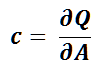
Here c is the dynamic wave celerity and B is the top width at normal depth for discharge Q. This highly efficient and accurate flow routing algorithm is used by InfoSewerH20Map Sewer Pro to track the spatial and temporal variation of flows throughout the collection system.

In this method (a.k.a., one sweep explicit solution method), the network flow dynamic equations are formulated by using an explicit finite difference scheme such that the flow depth, discharge, or velocity at a given location and the current time can be solved explicitly from the known information at the previous locations at the same time level, as well as known information at the previous time level. Thus, the solution is obtained segment by segment, pipe by pipe, over a given time interval for the entire sewer network before progressing to the next interval for another sweep of individual solutions of the network flow equations for the entire network. A variable time step approach (based on the Courant number

is used to minimize numerical dispersion and ensure robustness and stability of the numerical scheme. Complex flow attenuation calculations can be explicitly carried out to more accurately simulate the movement and transformation of sanitary sewer flows in the collection system.

An excellent review and comparison between simulated and observed hydrographs of the various numerical methods for solving unsteady flow in simple and compound channels was presented by Chatila (Chatila 2003). In terms of overall performance, the Muskingum unsteady solution scheme compared favorably and proved to be a simple and reliable method avoiding complicated mathematical and numerical computations for the cases considered.

Flooding at manholes and wet-wells in InfoSewerH20Map Sewer Pro is not modeled during an extended period dynamic simulation. Instead, the flows at the flooded structures are conserved and are not lost by the occurrence of flooding at the manholes. In actual flooding situations, flows may be diverted away from the flooded structures and out of the sewer collection system. However, a surcharged pipe or manhole is generally an indication of poor hydraulic performance of the sewer system. InfoSewer/Pro assumes that the downstream pipes of flooded manholes are flowing full.

Sanitary sewer systems are typically designed to flow less than full and have an upper pressure limit of 4 to 6 psi. Sewer systems operating under pressurized flow condition may run the risk of violating local, state, and federal health codes. The USEPA regulations would also be in violation if raw sewage were discharged into the ground, potentially affecting groundwater. For these reasons, pressurized flows in sanitary sewers not designed to sustain pressures can be dangerous and in some cases can present an unlawful activity.

Surcharge

Sewer pipes can flow full with water under pressure, which is often known as surcharge flow. Surcharge flow occurs in under-designed pipes (or under extreme flows) when the flow rate Q exceeds the full pipe capacity Qf .

Flow conditions are unstable at the transition between open-channel (free surface) flow and full pipe flow. A wave or surge can induce full flow in the pipe in the unstable range. Surcharge in sewer pipes is modeled in InfoSewerH20Map Sewer Pro using energy and continuity principles. The energy equation between sections 1 and 2 in a pipe can be written as:

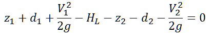
Here z denotes the invert elevation; d represents the water depth; and HL designates the head loss between sections 1 and 2. The energy equation is used to determine the difference in hydraulic grade line elevation (which is added at the upstream manholes) needed to pass downstream flows under the surcharge condition.

The procedure for analyzing surcharge in sewer pipes is illustrated using the figure below as a reference.

Assuming that pipe 4 (between manholes 4 and 5) is under-designed, Q4 will exceed its full flow capacity and the hydraulic grade line at manhole 4 will increase based on energy consideration to allow Q4 to pass through pipe 4 (note that water always flows from higher to lower energy) as continuity must be satisfied. This forces the hydraulic grade line at manhole 3 to increase in order for Q3 to pass through pipe 3. The procedure continues upstream until the slope of the energy grade line needed to transport the flow allows open-channel flow condition to occur in the pipe. The projected hydraulic grade line will then intersect the uniform water surface flow to complete the backwater curve.

The energy equation is also used to model the flow in siphons, which can occur in adverse pipes. InfoSewer assumes that the siphon flows full, with a continuous liquid column throughout it. This image shows how an adverse sloped link infoSewer looks

Flow Attenuation

When a flow hydrograph is injected and propagates downstream in sewer pipes the bulk of the water will normally travel slower than its induced disturbance or wave. That is, if the water is injected with a tracer then the tracer lags behind the disturbance. The speed of the disturbance depends on parameters such as depth, width and flow velocity. This disturbance will tend to flatten, or spread out, the peak flow in the downstream direction along the sewer pipes.

Flow attenuation in a sewer system is defined as the process of reducing the peak flow rate by redistributing the same volume of flow over a longer period of time as a result of friction (resistance), internal storage and diffusion along the sewer pipes. InfoSewerH20Map Sewer Pro uses the distributed Muskingum-Cunge flow routing method based on diffusion analogy, which is capable of accurately predicting hydrograph attenuation or peak flow damping effects (peak subsidence). The method is attractive since the routing parameters can be directly calculated as a function of pipe and flow properties, is applicable for a wide range of flow conditions, and does not require calibration or any iterative scheme. The Muskingum coefficients are derived from the pipe diameter, length, discharge, dynamic wave celerity, and slope of the flow. The magnitude of attenuation depends on parameters such as the peak discharge, the curvature of the hydrograph, and the width of flow. An example of flow attenuation process as a hydrograph is routed through a sewer system is illustrated in the figure below.

Hydrograph Aggregation/Flow Accumulation

Proper aggregation of multiple hydrographs with distinct time steps is essential in a sewer collection system as the flows are routed in both time and space. Aggregation normally occurs when laterals are merging around manholes and wet-wells. This can create offset of time-steps, which can affect accurate determination of flow peaks and volumes. InfoSewerH20Map SewerPro utilizes a highly accurate dynamic hydrograph aggregation method that allows preservation of both flow peaks and flow volumes when multiple hydrographs with different time steps are added. The method is Lagrangian in nature and tracks the hydrograph ordinates as they are transported along the sewer pipes and mix together at manholes and wet-wells. A variable time step is used to minimize numerical dispersion, enhance stability, and maximize computational efficiency. See the User Guide for more information on Extended Period Simulations.